Archive
O’Reilly book deal signed for “Doing Data Science”
I’m very happy to say I just signed a book contract with my co-author, Rachel Schutt, to publish a book with O’Reilly called Doing Data Science.
The book will be based on the class Rachel is giving this semester at Columbia which I’ve been blogging about here.
For those of you who’ve been reading along for free as I’ve been blogging it, there might not be a huge incentive to buy it, but I can promise you more and better math, more explicit usable formulas, some sample code, and an overall better and more thought-out narrative.
It’s supposed to be published in May with a possible early release coming up at the end of February, in time for the O’Reilly Strata Santa Clara conference, where Rachel will be speaking about it and about other stuff curriculum related. Hopefully people will pick it up in time to teach their data science courses in Fall 2013.
Speaking of Rachel, she’s also been selected to give a TedXWomen talk at Barnard on December 1st, which is super exciting. She’s talking about advocating for the social good using data. Unfortunately the event is invitation-only, otherwise I’d encourage you all to go and hear her words of wisdom. Update: word on the street is that it will be video-taped.
Columbia Data Science course, week 11: Estimating causal effects
The week in Rachel Schutt’s Data Science course at Columbia we had Ori Stitelman, a data scientist at Media6Degrees.
We also learned last night of a new Columbia course: STAT 4249 Applied Data Science, taught by Rachel Schutt and Ian Langmore. More information can be found here.
Ori’s background
Ori got his Ph.D. in Biostatistics from UC Berkeley after working at a litigation consulting firm. He credits that job with allowing him to understand data through exposure to tons of different data sets; since his job involved creating stories out of data to let experts testify at trials, e.g. for asbestos. In this way Ori developed his data intuition.
Ori worries that people ignore this necessary data intuition when they shove data into various algorithms. He thinks that when their method converges, they are convinced the results are therefore meaningful, but he’s here today to explain that we should be more thoughtful than that.
It’s very important when estimating causal parameters, Ori says, to understand the data-generating distributions and that involves gaining subject matter knowledge that allows you to understand if you necessary assumptions are plausible.
Ori says the first step in a data analysis should always be to take a step back and figure out what you want to know, write that down, and then find and use the tools you’ve learned to answer those directly. Later of course you have to decide how close you came to answering your original questions.
Thought Experiment
Ori asks, how do you know if your data may be used to answer your question of interest? Sometimes people think that because they have data on a subject matter then you can answer any question.
Students had some ideas:
- You need coverage of your parameter space. For example, if you’re studying the relationship between household income and holidays but your data is from poor households, then you can’t extrapolate to rich people. (Ori: but you could ask a different question)
- Causal inference with no timestamps won’t work.
- You have to keep in mind what happened when the data was collected and how that process affected the data itself
- Make sure you have the base case: compared to what? If you want to know how politicians are affected by lobbyists money you need to see how they behave in the presence of money and in the presence of no money. People often forget the latter.
- Sometimes you’re trying to measure weekly effects but you only have monthly data. You end up using proxies. Ori: but it’s still good practice to ask the precise question that you want, then come back and see if you’ve answered it at the end. Sometimes you can even do a separate evaluation to see if something is a good proxy.
- Signal to noise ratio is something to worry about too: as you have more data, you can more precisely estimate a parameter. You’d think 10 observations about purchase behavior is not enough, but as you get more and more examples you can answer more difficult questions.
Ori explains confounders with a dating example
Frank has an important decision to make. He’s perusing a dating website and comes upon a very desirable woman – he wants her number. What should he write in his email to her? Should he tell her she is beautiful? How do you answer that with data?
You could have him select a bunch of beautiful women and half the time chosen at random, tell them they’re beautiful. Being random allows us to assume that the two groups have similar distributions of various features (not that’s an assumption).
Our real goal is to understand the future under two alternative realities, the treated and the untreated. When we randomize we are making the assumption that the treated and untreated populations are alike.
OK Cupid looked at this and concluded:

But note:
- It could say more about the person who says “beautiful” than the word itself. Maybe they are otherwise ridiculous and overly sappy?
- The recipients of emails containing the word “beautiful” might be special: for example, they might get tons of email, which would make it less likely for Frank to get any response at all.
- For that matter, people may be describing themselves as beautiful.
Ori points out that this fact, that she’s beautiful, affects two separate things:
- whether Frank uses the word “beautiful” or not in his email, and
- the outcome (i.e. whether Frank gets the phone number).
For this reason, the fact that she’s beautiful qualifies as a confounder. The treatment is Frank writing “beautiful” in his email.
Causal graphs
Denote by 
Denote by 
Denote by 
We are forming the following causal graph:

In a causal graph, each arrow means that the ancestor is a cause of the descendent, where ancestor is the node the arrow is coming out of and the descendent is the node the arrow is going into (see this book for more).
In our example with Frank, the arrow from beauty means that the woman being beautiful is a cause of Frank writing “beautiful” in the message. Both the man writing “beautiful” and and the woman being beautiful are direct causes of her probability to respond to the message.
Setting the problem up formally
The building blocks in understanding the above causal graph are:
- Ask question of interest.
- Make causal assumptions (denote these by
).
- Translate question into a formal quantity (denote this by
).
- Estimate quantity (denote this by
).
We need domain knowledge in general to do this. We also have to take a look at the data before setting this up, for example to make sure we may make the
Positivity Assumption. We need treatment (i.e. data) in all strata of things we adjust for. So if think gender is a confounder, we need to make sure we have data on women and on men. If we also adjust for age, we need data in all of the resulting bins.
Asking causal questions
What is the effect of ___ on ___?
This is the natural form of a causal question. Here are some examples:
- What is the effect of advertising on customer behavior?
- What is the effect of beauty on getting a phone number?
- What is the effect of censoring on outcome? (censoring is when people drop out of a study)
- What is the effect of drug on time until viral failure?, and the general case
- What is the effect of treatment on outcome?
Look, estimating causal parameters is hard. In fact the effectiveness of advertising is almost always ignored because it’s so hard to measure. Typically people choose metrics of success that are easy to estimate but don’t measure what they want! Everyone makes decision based on them anyway because it’s easier. This results in people being rewarded for finding people online who would have converted anyway.
Accounting for the effect of interventions
Thinking about that, we should be concerned with the effect of interventions. What’s a model that can help us understand that effect?
A common approach is the (randomized) A/B test, which involves the assumption that two populations are equivalent. As long as that assumption is pretty good, which it usually is with enough data, then this is kind of the gold standard.
But A/B tests are not always possible (or they are too expensive to be plausible). Often we need to instead estimate the effects in the natural environment, but then the problem is the guys in different groups are actually quite different from each other.
So, for example, you might find you showed ads to more people who are hot for the product anyway; it wouldn’t make sense to test the ad that way without adjustment.
The game is then defined: how do we adjust for this?
The ideal case
Similar to how we did this last week, we pretend for now that we have a “full” data set, which is to say we have god-like powers and we know what happened under treatment as well as what would have happened if we had not treated, as well as vice-versa, for every agent in the test.
Denote this full data set by


denotes the binary outcome if treated, and
denotes the binary outcome if untreated.
As a baseline check: if we observed this full data structure how would we measure the effect of A on Y? In that case we’d be all-powerful and we would just calculate:

Note that, since 

This would be calculating how much more likely someone is to convert if they see an ad.
Note these are outcomes you can really do stuff with. If you know people convert at 30% versus 10% in the presence of an ad, that’s real information. Similarly if they convert 3 times more often.
In reality people use silly stuff like log odds ratios, which nobody understands or can interpret meaningfully.
The ideal case with functions
In reality we don’t have god-like powers, and we have to make do. We will make a bunch of assumptions. First off, denote by 


i.e. the attributes
i.e. the treatment depends in a nice way on some exogenous variables as well the attributes we know about living in
i.e. the outcome is just a function of the treatment, the attributes, and some exogenous variables.
Note the various
But we want to intervene on this causal graph as though it’s the intervention we actually want to make. i.e. what’s the effect of treatment
Let’s look at this from the point of view of the joint distribution 
- the probability of a woman being beautiful,
- the probability that Frank writes and email to a her saying that she’s beautiful, and
- the probability that Frank gets her phone number.
What we really care about though is the distribution under intervention:
i.e. the probability knowing someone either got treated or not. To answer our question, we manipulate the value of 
Assumptions
We are making a “Consistency Assumption / SUTVA” which can be expressed like this:
![]()
We have also assumed that we have no unmeasured confounders, which can be expressed thus:

We are also assuming positivity, which we discussed above.
Down to brass tacks
We only have half the information we need. We need to somehow map the stuff we have to the full data set as defined above. We make use of the following identity:

Recall we want to estimate 

We’re going to discuss three methods to estimate this quantity, namely:
- MLE-based substitution estimator (MLE),
- Inverse probability estimators (IPTW),
- Double robust estimating equations (A-IPTW)
For the above models, it’s useful to think of there being two machines, called 

IPTW
In this method, which is also called importance sampling, we weight individuals that are unlikely to be shown an ad more than those likely. In other words, we up-sample in order to generate the distribution, to get the estimation of the actual effect.
To make sense of this, imagine that you’re doing a survey of people to see how they’ll vote, but you happen to do it at a soccer game where you know there are more young people than elderly people. You might want to up-sample the elderly population to make your estimate.
This method can be unstable if there are really small sub-populations that you’re up-sampling, since you’re essentially multiplying by a reciprocal.
The formula in IPTW looks like this:

Note the formula depends on the
In words, when 

MLE
This method is based on the
This method is straight-forward: shove everyone in the machine and predict how the outcome would look under both treatment and non-treatment conditions, and take difference.
Note we don’t know anything about the underlying machine $latex Q$. It could be a logistic regression.
Get ready to get worried: A-IPTW
What if our machines are broken? That’s when we bring in the big guns: double robust estimators.
They adjust for confounding through the two machines we have on hand, 

and

Note: you are still screwed if both machines are broken. In some sense with a double robust estimator you’re hedging your bet.
“I’m glad you’re worried because I’m worried too.” – Ori
Simulate and test
I’ve shown you 3 distinct methods that estimate effects in observational studies. But they often come up with different answers. We set up huge simulation studies with known functions, i.e. where we know the functional relationships between everything, and then tried to infer those using the above three methods as well as a fourth method called TMLE (targeted maximal likelihood estimation).
As a side note, Ori encourages everyone to simulate data.
We wanted to know, which methods fail with respect to the assumptions? How well do the estimates work?
We started to see that IPTW performs very badly when you’re adjusting by very small thing. For example we found that the probability of someone getting sick is 132. That’s not between 0 and 1, which is not good. But people use these methods all the time.
Moreover, as things get more complicated with lots of nodes in our causal graph, calculating stuff over long periods of time, populations get sparser and sparser and it has an increasingly bad effect when you’re using IPTW. In certain situations your data is just not going to give you a sufficiently good answer.
Causal analysis in online display advertising
An overview of the process:
- We observe people taking actions (clicks, visits to websites, purchases, etc.).
- We use this observed data to build list of “prospects” (people with a liking for the brand).
- We subsequently observe same user during over the next few days.
- The user visits a site where a display ad spot exists and bid requests are made.
- An auction is held for display spot.
- If the auction is won, we display the ad.
- We observe the user’s actions after displaying the ad.
But here’s the problem: we’ve instituted confounders – if you find people who convert highly they think you’ve done a good job. In other words, we are looking at the treated without looking at the untreated.
We’d like to ask the question, what’s the effect of display advertising on customer conversion?
As a practical concern, people don’t like to spend money on blank ads. So A/B tests are a hard sell.
We performed some what-if analysis stipulated on the assumption that the group of users that sees ad is different. Our process was as follows:
- Select prospects that we got a bid request for on day 0
- Observe if they were treated on day 1. For those treated set
and those not treated set
collect attributes
- Create outcome window to be the next five days following treatment; observe if outcome event occurs (visit to the website whose ad was shown).
- Estimate model parameters using the methods previously described (our three methods plus TMLE).

Here are some results:

Note results vary depending on the method. And there’s no way to know which method is working the best. Moreover, this is when we’ve capped the size of the correction in the IPTW methods. If we don’t then we see ridiculous results:

Data science in the natural sciences
This is a guest post written by Chris Wiggins, crossposted from strata.oreilly.com.
I find myself having conversations recently with people from increasingly diverse fields, both at Columbia and in local startups, about how their work is becoming “data-informed” or “data-driven,” and about the challenges posed by applied computational statistics or big data.
A view from health and biology in the 1990s
In discussions with, as examples, New York City journalists, physicists, or even former students now working in advertising or social media analytics, I’ve been struck by how many of the technical challenges and lessons learned are reminiscent of those faced in the health and biology communities over the last 15 years, when these fields experienced their own data-driven revolutions and wrestled with many of the problems now faced by people in other fields of research or industry.
It was around then, as I was working on my PhD thesis, that sequencing technologies became sufficient to reveal the entire genomes of simple organisms and, not long thereafter, the first draft of the human genome. This advance in sequencing technologies made possible the “high throughput” quantification of, for example,
- the dynamic activity of all the genes in an organism; or
- the set of all protein-protein interactions in an organism; or even
- statistical comparative genomics revealing how small differences in genotype correlate with disease or other phenotypes.
These advances required formation of multidisciplinary collaborations, multi-departmental initiatives, advances in technologies for dealing with massive datasets, and advances in statistical and mathematical methods for making sense of copious natural data.
The fourth paradigm
This shift wasn’t just a series of technological advances in biological research; the more important change was a realization that research in which data vastly outstrip our ability to posit models is qualitatively different. Much of science for the last three centuries advanced by deriving simple models from first principles — models whose predictions could then be compared with novel experiments. In modeling complex systems for which the underlying model is not yet known but for which data are abundant, however, as in systems biology or social network analysis, one may turn this process on its head by using the data to learn not only parameters of a single model but to select which among many or an infinite number of competing models is favored by the data. Just over a half-decade ago, the computer scientist Jim Gray described this as a “fourth paradigm” of science, after experimental, theoretical, and computational paradigms. Gray predicted that every sector of human endeavor will soon emulate biology’s example of identifying data-driven research and modeling as a distinct field.
In the years since then we’ve seen just that. Examples include data-driven social sciences (often leveraging the massive data now available through social networks) and even data-driven astronomy (cf., Astronomy.net). I’ve personally enjoyed seeing many students from Columbia’s School of Engineering and Applied Science (SEAS), trained in applications of big data to biology, go on to develop and apply data-driven models in these fields. As one example, a recent SEAS PhD student spent a summer as a “hackNY Fellow” applying machine learning methods at the data-driven dating NYC startup OKCupid. [Disclosure: I’m co-founder and co-president of hackNY.] He’s now applying similar methods to population genetics as a postdoctoral researcher at the University of Chicago. These students, often with job titles like “data scientist,” are able to translate to other fields, or even to the “real world” of industry and technology-driven startups, methods needed in biology and health for making sense of abundant natural data.
Data science: Combining engineering and natural sciences
In my research group, our work balances “engineering” goals, e.g., developing models that can make accurate quantitative predictions, with “natural science” goals, meaning building models that are interpretable to our biology and clinical collaborators, and which suggest to them what novel experiments are most likely to reveal the workings of natural systems. For example:
- We’ve developed machine-learning methods for modeling the expression of genes — the “on-off” state of the tens of thousands of individual processes your cells execute — by combining sequence data with microarray expression data. These models reveal which genes control which other genes, via what important sequence elements.
- We’ve analyzed large biological protein networks and shown how statistical signatures reveal what evolutionary laws can give rise to such graphs.
- In collaboration with faculty at Columbia’s chemistry department and NYU’s medical school, we’ve developed hierarchical Bayesian inference methods that can automate the analysis of thousands of time series data from single molecules. These techniques can identify the best model from models of varying complexity, along with the kinetic and biophysical parameters of interest to the chemist and clinician.
- Our current projects include, in collaboration with experts at Columbia’s medical school in pathogenic viral genomics, using machine learning methods to reveal whether a novel viral sequence may be carcinogenic or may lead to a pandemic. This research requires an abundant corpus of training data as well as close collaboration with the domain experts to ensure that the models exploit — and are interpretable in light of — the decades of bench work that has revealed what we now know of viral pathogenic mechanisms.
Throughout, our goals balance building models that are not only predictive but interpretable, e.g., revealing which sequence elements convey carcinogenicity or permit pandemic transmissibility.
Data science in health
More generally, we can apply big data approaches not only to biological examples as above but also to health data and health records. These approaches offer the possibility of, for example, revealing unknown lethal drug-drug interactions or forecasting future patient health problems; such models could have consequences for both public health policies and individual patent care. As one example, the Heritage Health Prize is a $3 million challenge ending in April 2013 “to identify patients who will be admitted to a hospital within the next year, using historical claims data.” Researchers at Columbia, both in SEAS and at Columbia’s medical school, are building the technologies needed for answering such big questions from big data.
The need for skilled data scientists
In 2011, the McKinsey Global Institute estimated that between 140,000 and 190,000 additional data scientistswill need to be trained by 2018 in order to meet the increased demand in academia and industry in the United States alone. The multidisciplinary skills required for data science applied to such fields as health and biology will include:
- the computational skills needed to work with large datasets usually shared online;
- the ability to format these data in a way amenable to mathematical modeling;
- the curiosity to explore these data to identify what features our models may be built on;
- the technical skills which apply, extend, and validate statistical and machine learning methods; and most importantly,
- the ability to visualize, interpret, and communicate the resulting insights in a way which advances science. (As the mathematician Richard Hamming said, “The purpose of computing is insight, not numbers.”)
More than a decade ago the statistician William Cleveland, then at Bell Labs, coined the term “data science” for this multidisciplinary set of skills and envisioned a future in which these skills would be needed for more fields of technology. The term has had a recent explosion in usage as more and more fields — both in academia and in industry — are realizing precisely this future.
Medical research needs an independent modeling panel
I am outraged this morning.
I spent yesterday morning writing up David Madigan’s lecture to us in the Columbia Data Science class, and I can hardly handle what he explained to us: the entire field of epidemiological research is ad hoc.
This means that people are taking medication or undergoing treatments that may do they harm and probably cost too much because the researchers’ methods are careless and random.
Of course, sometimes this is intentional manipulation (see my previous post on Vioxx, also from an eye-opening lecture by Madigan). But for the most part it’s not. More likely it’s mostly caused by the human weakness for believing in something because it’s standard practice.
In some sense we knew this already. How many times have we read something about what to do for our health, and then a few years later read the opposite? That’s a bad sign.
And although the ethics are the main thing here, the money is a huge issue. It required $25 million dollars for Madigan and his colleagues to implement the study on how good our current methods are at detecting things we already know. Turns out they are not good at this – even the best methods, which we have no reason to believe are being used, are only okay.
Okay, $25 million dollars is a lot, but then again there are literally billions of dollars being put into the medical trials and research as a whole, so you might think that the “due diligence” of such a large industry would naturally get funded regularly with such sums.
But you’d be wrong. Because there’s no due diligence for this industry, not in a real sense. There’s the FDA, but they are simply not up to the task.
One article I linked to yesterday from the Stanford Alumni Magazine, which talked about the work of John Ioannidis (I blogged about his work here called “Why Most Published Research Findings Are False“), summed the situation up perfectly (emphasis mine):
When it comes to the public’s exposure to biomedical research findings, another frustration for Ioannidis is that “there is nobody whose job it is to frame this correctly.” Journalists pursue stories about cures and progress—or scandals—but they aren’t likely to diligently explain the fine points of clinical trial bias and why a first splashy result may not hold up. Ioannidis believes that mistakes and tough going are at the essence of science. “In science we always start with the possibility that we can be wrong. If we don’t start there, we are just dogmatizing.”
It’s all about conflict of interest, people. The researchers don’t want their methods examined, the pharmaceutical companies are happy to have various ways to prove a new drug “effective”, and the FDA is clueless.
Another reason for an AMS panel to investigate public math models. If this isn’t in the public’s interest I don’t know what is.
Columbia Data Science course, week 10: Observational studies, confounders, epidemiology
This week our guest lecturer in the Columbia Data Science class was David Madigan, Professor and Chair of Statistics at Columbia. He received a bachelors degree in Mathematical Sciences and a Ph.D. in Statistics, both from Trinity College Dublin. He has previously worked for AT&T Inc., Soliloquy Inc., the University of Washington, Rutgers University, and SkillSoft, Inc. He has over 100 publications in such areas as Bayesian statistics, text mining, Monte Carlo methods, pharmacovigilance and probabilistic graphical models.
So Madigan is an esteemed guest, but I like to call him an “apocalyptic leprechaun”, for reasons which you will know by the end of this post. He’s okay with that nickname, I asked his permission.
Madigan came to talk to us about observation studies, of central importance in data science. He started us out with this:
Thought Experiment
We now have detailed, longitudinal medical data on tens of millions of patients. What can we do with it?
To be more precise, we have tons of phenomenological data: this is individual, patient-level medical record data. The largest of the databases has records on 80 million people: every prescription drug, every condition ever diagnosed, every hospital or doctor’s visit, every lab result, procedures, all timestamped.
But we still do things like we did in the Middle Ages; the vast majority of diagnosis and treatment is done in a doctor’s brain. Can we do better? Can you harness these data to do a better job delivering medical care?
Students responded:
1) There was a prize offered on Kaggle, called “Improve Healthcare, Win $3,000,000.” predicting who is going to go to the hospital next year. Doesn’t that give us some idea of what we can do?
Madigan: keep in mind that they’ve coarsened the data for proprietary reasons. Hugely important clinical problem, especially as a healthcare insurer. Can you intervene to avoid hospitalizations?
2) We’ve talked a lot about the ethical uses of data science in this class. It seems to me that there are a lot of sticky ethical issues surrounding this 80 million person medical record dataset.
Madigan: Agreed! What nefarious things could we do with this data? We could gouge sick people with huge premiums, or we could drop sick people from insurance altogether. It’s a question of what, as a society, we want to do.
What is modern academic statistics?
Madigan showed us Drew Conway’s Venn Diagram that we’d seen in week 1:
 Madigan positioned the modern world of the statistician in the green and purple areas.
It used to be the case, say 20 years ago, according to Madigan, that academic statistician would either sit in their offices proving theorems with no data in sight (they wouldn’t even know how to run a t-test) or sit around in their offices and dream up a new test, or a new way of dealing with missing data, or something like that, and then they’d look around for a dataset to whack with their new method. In either case, the work of an academic statistician required no domain expertise.
Nowadays things are different. The top stats journals are more deep in terms of application areas, the papers involve deep collaborations with people in social sciences or other applied sciences. Madigan is setting an example tonight by engaging with the medical community.
Madigan went on to make a point about the modern machine learning community, which he is or was part of: it’s a newish academic field, with conferences and journals, etc., but is characterized by what stats was 20 years ago: invent a method, try it on datasets. In terms of domain expertise engagement, it’s a step backwards instead of forwards.
Comments like the above make me love Madigan.
Very few academic statisticians have serious hacking skills, with Mark Hansen being an unusual counterexample. But if all three is what’s required to be called data science, then I’m all for data science, says Madigan.
Madigan’s timeline
Madigan went to college in 1980, specialized on day 1 on math for five years. In final year, he took a bunch of stats courses, and learned a bunch about computers: pascal, OS, compilers, AI, database theory, and rudimentary computing skills. Then came 6 years in industry, working at an insurance company and a software company where he specialized in expert systems.
It was a mainframe environment, and he wrote code to price insurance policies using what would now be described as scripting languages. He also learned about graphics by creating a graphic representation of a water treatment system. He learned about controlling graphics cards on PC’s, but he still didn’t know about data.
Then he got a Ph.D. and went into academia. That’s when machine learning and data mining started, which he fell in love with: he was Program Chair of the KDD conference, among other things, before he got disenchanted. He learned C and java, R and S+. But he still wasn’t really working with data yet.
He claims he was still a typical academic statistician: he had computing skills but no idea how to work with a large scale medical database, 50 different tables of data scattered across different databases with different formats.
In 2000 he worked for AT&T labs. It was an “extreme academic environment”, and he learned perl and did lots of stuff like web scraping. He also learned awk and basic unix skills.
It was life altering and it changed everything: having tools to deal with real data rocks! It could just as well have been python. The point is that if you don’t have the tools you’re handicapped. Armed with these tools he is afraid of nothing in terms of tackling a data problem.
In Madigan’s opinion, statisticians should not be allowed out of school unless they know these tools.
He then went to a internet startup where he and his team built a system to deliver real-time graphics on consumer activity.
Since then he’s been working in big medical data stuff. He’s testified in trials related to medical trials, which was eye-opening for him in terms of explaining what you’ve done: “If you’re gonna explain logistical regression to a jury, it’s a different kind of a challenge than me standing here tonight.” He claims that super simple graphics help.
Carrotsearch
As an aside he suggests we go to this website, called carrotsearch, because there’s a cool demo on it.
What is an observational study?
Madigan defines it for us:
An observational study is an empirical study in which the objective is to elucidate cause-and-effect relationships in which it is not feasible to use controlled experimentation.
In tonight’s context, it will involve patients as they undergo routine medical care. We contrast this with designed experiment, which is pretty rare. In fact, Madigan contends that most data science activity revolves around observational data. Exceptions are A/B tests. Most of the time, the data you have is what you get. You don’t get to replay a day on the market where Romney won the presidency, for example.
Observational studies are done in contexts in which you can’t do experiments, and they are mostly intended to elucidate cause-and-effect. Sometimes you don’t care about cause-and-effect, you just want to build predictive models. Madigan claims there are many core issues in common with the two.
Here are some examples of tests you can’t run as designed studies, for ethical reasons:
- smoking and heart disease (you can’t randomly assign someone to smoke)
- vitamin C and cancer survival
- DES and vaginal cancer
- aspirin and mortality
- cocaine and birthweight
- diet and mortality
Pitfall #1: confounders
There are all kinds of pitfalls with observational studies.
For example, look at this graph, where you’re finding a best fit line to describe whether taking higher doses of the “bad drug” is correlated to higher probability of a heart attack:

It looks like, from this vantage point, the more drug you take the fewer heart attacks you have. But there are two clusters, and if you know more about those two clusters, you find the opposite conclusion:

Note this picture was rigged it so the issue is obvious. This is an example of a “confounder.” In other words, the aspirin-taking or non-aspirin-taking of the people in the study wasn’t randomly distributed among the people, and it made a huge difference.
It’s a general problem with regression models on observational data. You have no idea what’s going on.
Madigan: “It’s the wild west out there.”
Wait, and it gets worse. It could be the case that within each group there males and females and if you partition by those you see that the more drugs they take the better again. Since a given person either is male or female, and either takes aspirin or doesn’t, this kind of thing really matters.
This illustrates the fundamental problem in observational studies, which is sometimes called Simpson’s Paradox.
[Remark from someone in the class: if you think of the original line as a predictive model, it’s actually still the best model you can obtain knowing nothing more about the aspirin-taking habits or genders of the patients involved. The issue here is really that you’re trying to assign causality.]
The medical literature and observational studies
As we may not be surprised to hear, medical journals are full of observational studies. The results of these studies have a profound effect on medical practice, on what doctors prescribe, and on what regulators do.
For example, in this paper, entitled “Oral bisphosphonates and risk of cancer of oesophagus, stomach, and colorectum: case-control analysis within a UK primary care cohort,” Madigan report that we see the very same kind of confounding problem as in the above example with aspirin. The conclusion of the paper is that the risk of cancer increased with 10 or more prescriptions of oral bisphosphonates.
It was published on the front page of new york times, the study was done by a group with no apparent conflict of interest and the drugs are taken by millions of people. But the results were wrong.
There are thousands of examples of this, it’s a major problem and people don’t even get that it’s a problem.
Randomized clinical trials
One possible way to avoid this problem is randomized studies. The good news is that randomization works really well: because you’re flipping coins, all other factors that might be confounders (current or former smoker, say) are more or less removed, because I can guarantee that smokers will be fairly evenly distributed between the two groups if there are enough people in the study.
The truly brilliant thing about randomization is that randomization matches well on the possible confounders you thought of, but will also give you balance on the 50 million things you didn’t think of.
So, although you can algorithmically find a better split for the ones you thought of, that quite possible wouldn’t do as well on the other things. That’s why we really do it randomly, because it does quite well on things you think of and things you don’t.
But there’s bad news for randomized clinical trials as well. First off, it’s only ethically feasible if there’s something called clinical equipoise, which means the medical community really doesn’t know which treatment is better. If you know have reason to think treating someone with a drug will be better for them than giving them nothing, you can’t randomly not give people the drug.
The other problem is that they are expensive and cumbersome. It takes a long time and lots of people to make a randomized clinical trial work.
In spite of the problems, randomized clinical trials are the gold standard for elucidating cause-and-effect relationships.
Rubin causal model
The Rubin causal model is a mathematical framework for understanding what information we know and don’t know in observational studies.
It’s meant to investigate the confusion when someone says something like “I got lung cancer because I smoked”. Is that true? If so, you’d have to be able to support the statement, “If I hadn’t smoked I wouldn’t have gotten lung cancer,” but nobody knows that for sure.
Define:
to be the treatment applied to unit
(0 = control, 1= treatment),
to be the response for unit
,
to be the response for unit
.
Then the unit level causal effect is 

Example: 
Of course, on a population level we do know how to infer that there are quite a few “1”‘s among the population, but we will never be able to assign a given individual that number.
This is sometimes called the fundamental problem of causal inference.
Confounding and Causality
Let’s say we have a population of 100 people that takes some drug, and we screen them for cancer. Say 30 out of them get cancer, which gives them a cancer rate of 0.30. We want to ask the question, did the drug cause the cancer?
To answer that, we’d have to know what would’ve happened if they hadn’t taken the drug. Let’s play God and stipulate that, had they not taken the drug, we would have seen 20 get cancer, so a rate of 0.20. We typically say the causal effect is the ration of these two numbers (i.e. the increased risk of cancer), so 1.5.
But we don’t have God’s knowledge, so instead we choose another population to compare this one to, and we see whether they get cancer or not, whilst not taking the drug. Say they have a natural cancer rate of 0.10. Then we would conclude, using them as a proxy, that the increased cancer rate is the ratio 0.30 to 0.10, so 3. This is of course wrong, but the problem is that the two populations have some underlying differences that we don’t account for.
If these were the “same people”, down to the chemical makeup of each other molecules, this “by proxy” calculation would work of course.
The field of epidemiology attempts to adjust for potential confounders. The bad news is that it doesn’t work very well. One reason is that they heavily rely on stratification, which means partitioning the cases into subcases and looking at those. But there’s a problem here too.
Stratification can introduce confounding.
The following picture illustrates how stratification could make the underlying estimates of the causal effects go from good to bad:

In the top box, the values of b and c are equal, so our causal effect estimate is correct. However, when you break it down by male and female, you get worse estimates of causal effects.
The point is, stratification doesn’t just solve problems. There are no guarantees your estimates will be better if you stratify and all bets are off.
What do people do about confounding things in practice?
In spite of the above, experts in this field essentially use stratification as a major method to working through studies. They deal with confounding variables by essentially stratifying with respect to them. So if taking aspirin is believed to be a potential confounding factor, they stratify with respect to it.
For example, with this study, which studied the risk of venous thromboembolism from the use of certain kinds of oral contraceptives, the researchers chose certain confounders to worry about and concluded the following:
After adjustment for length of use, users of oral contraceptives were at least twice the risk of clotting compared with user of other kinds of oral contraceptives.
This report was featured on ABC, and it was a big hoo-ha.
Madigan asks: wouldn’t you worry about confounding issues like aspirin or something? How do you choose which confounders to worry about? Wouldn’t you worry that the physicians who are prescribing them are different in how they prescribe? For example, might they give the newer one to people at higher risk of clotting?
Another study came out about this same question and came to a different conclusion, using different confounders. They adjusted for a history of clots, which makes sense when you think about it.
This is an illustration of how you sometimes forget to adjust for things, and the outputs can then be misleading.
What’s really going on here though is that it’s totally ad hoc, hit or miss methodology.
Another example is a study on oral bisphosphonates, where they adjusted for smoking, alcohol, and BMI. But why did they choose those variables?
There are hundreds of examples where two teams made radically different choices on parallel studies. We tested this by giving a bunch of epidemiologists the job to design 5 studies at a high level. There was zero consistency. And an addition problem is that luminaries of the field hear this and say: yeah yeah yeah but I would know the right way to do it.
Is there a better way?
Madigan and his co-authors examined 50 studies, each of which corresponds to a drug and outcome pair, e.g. antibiotics with GI bleeding.
They ran about 5,000 analyses for every pair. Namely, they ran every epistudy imaginable on, and they did this all on 9 different databases.
For example, they looked at ACE inhibitors (the drug) and swelling of the heart (outcome). They ran the same analysis on the 9 different standard databases, the smallest of which has records of 4,000,000 patients, and the largest of which has records of 80,000,000 patients.
In this one case, for one database the drug triples the risk of heart swelling, but for another database it seems to have a 6-fold increase of risk. That’s one of the best examples, though, because at least it’s always bad news – it’s consistent.
On the other hand, for 20 of the 50 pairs, you can go from statistically significant in one direction (bad or good) to the other direction depending on the database you pick. In other words, you can get whatever you want. Here’s a picture, where the heart swelling example is at the top:

Note: the choice of database is never discussed in any of these published epidemiology papers.
Next they did an even more extensive test, where they essentially tried everything. In other words, every time there was a decision to be made, they did it both ways. The kinds of decisions they tweaker were of the following types: which database you tested on, the confounders you accounted for, the window of time you care about examining (spoze they have a heart attack a week after taking the drug, is it counted? 6 months?)
What they saw was that almost all the studies can get either side depending on the choices.
Final example, back to oral bisphosphonates. A certain study concluded that it causes esophageal cancer, but two weeks later JAMA published a paper on same issue which concluded it is not associated to elevated risk of esophageal cancer. And they were even using the same database. This is not so surprising now for us.
OMOP Research Experiment
Here’s the thing. Billions upon billions of dollars are spent doing these studies. We should really know if they work. People’s lives depend on it.
Madigan told us about his “OMOP 2010.2011 Research Experiment”
They took 10 large medical databases, consisting of a mixture of claims from insurance companies and EHR (electronic health records), covering records of 200 million people in all. This is big data unless you talk to an astronomer.
They mapped the data to a common data model and then they implemented every method used in observational studies in healthcare. Altogether they covered 14 commonly used epidemiology designs adapted for longitudinal data. They automated everything in sight. Moreover, there were about 5000 different “settings” on the 14 methods.
The idea was to see how well the current methods do on predicting things we actually already know.
To locate things they know, they took 10 old drug classes: ACE inhibitors, beta blockers, warfarin, etc., and 10 outcomes of interest: renal failure, hospitalization, bleeding, etc.
For some of these the results are known. So for example, warfarin is a blood thinner and definitely causes bleeding. There were 9 such known bad effects.
There were also 44 known “negative” cases, where we are super confident there’s just no harm in taking these drugs, at least for these outcomes.
The basic experiment was this: run 5000 commonly used epidemiological analyses using all 10 databases. How well do they do at discriminating between reds and blues?
This is kind of like a spam filter test. We have training emails that are known spam, and you want to know how well the model does at detecting spam when it comes through.
Each of the models output the same thing: a relative risk (causal effect estimate) and an error.
This was an attempt to empirically evaluate how well does epidemiology work, kind of the quantitative version of John Ioannidis’s work. we did the quantitative thing to show he’s right.
Why hasn’t this been done before? There’s conflict of interest for epidemiology – why would they want to prove their methods don’t work? Also, it’s expensive, it cost $25 million dollars (of course that pales in comparison to the money being put into these studies). They bought all the data, made the methods work automatically, and did a bunch of calculations in the Amazon cloud. The code is open source.
In the second version, we zeroed in on 4 particular outcomes. Here’s the $25,000,000 ROC curve:

To understand this graph, we need to define a threshold, which we can start with at 2. This means that if the relative risk is estimated to be above 2, we call it a “bad effect”, otherwise call it a “good effect.” The choice of threshold will of course matter.
If it’s high, say 10, then you’ll never see a 10, so everything will be considered a good effect. Moreover these are old drugs and it wouldn’t be on the market. This means your sensitivity will be low, and you won’t find any real problem. That’s bad! You should find, for example, that warfarin causes bleeding.
There’s of course good news too, with low sensitivity, namely a zero false-positive rate.
What if you set the threshold really low, at -10? Then everything’s bad, and you have a 100% sensitivity but very high false positive rate.
As you vary the threshold from very low to very high, you sweep out a curve in terms of sensitivity and false-positive rate, and that’s the curve we see above. There is a threshold (say 1.8) for which your false positive rate is 30% and your sensitivity is 50%.
This graph is seriously problematic if you’re the FDA. A 30% false-positive rate is out of control. This curve isn’t good.
The overall “goodness” of such a curve is usually measured as the area under the curve: you want it to be one, and if your curve lies on diagonal the area is 0.5. This is tantamount to guessing randomly. So if your area under the curve is less than 0.5, it means your model is perverse.
The area above is 0.64. Moreover, of the 5000 analysis we ran, this is the single best analysis.
But note: this is the best if I can only use the same method for everything. In that case this is as good as it gets, and it’s not that much better than guessing.
But no epidemiology would do that!
So what they did next was to specialize the analysis to the database and the outcome. And they got better results: for the medicare database, and for acute kidney injury, their optimal model gives them an AUC of 0.92. They can achieve 80% sensitivity with a 10% false positive rate.

They did this using a cross-validation method. Different databases have different methods attached to them. One winning method is called “OS”, which compares within a given patient’s history (so compares times when patient was on drugs versus when they weren’t). This is not widely used now.
The epidemiologists in general don’t believe the results of this study.
If you go to http://elmo/omop.org, you can see the AUM for a given database and a given method.
Note the data we used was up to mid-2010. To update this you’d have to get latest version of database, and rerun the analysis. Things might have changed.
Moreover, an outcome for which nobody has any idea on what drugs cause what outcomes you’re in trouble. This only applies to when we have things to train on where we know the outcome pretty well.
Parting remarks
Keep in mind confidence intervals only account for sampling variability. They don’t capture bias at all. If there’s bias, the confidence interval or p-value can be meaningless.
What about models that epidemiologists don’t use? We have developed new methods as well (SCCS). we continue to do that, but it’s a hard problem.
Challenge for the students: we ran 5000 different analyses. Is there a good way of combining them to do better? weighted average? voting methods across different strategies?
Note the stuff is publicly available and might make a great Ph.D. thesis.
The zit model
When my mom turned 42, I was 12 and a total wise-ass. For her present I bought her a coffee mug that had on it the phrase “Things could be worse. You could be old and still have zits”, to tease her about her bad skin. Considering how obnoxious that was, she took it really well and drank out of the mug for years.
Well, I’m sure you can all see where this is going. I’m now 40 and I have zits. I was contemplating this in the bath yesterday, wondering if I’d ever get rid of my zits and wondering if taking long hot baths helps or not. They come and go, so it seems vaguely controllable.
Then I had a thought: well, I could collect data and see what helps. After all, I don’t always have zits. I could keep a diary of all the things that I think might affect the situation: what I eat (I read somewhere that eating cheese makes you have zits), how often I take baths vs. showers, whether I use zit cream, my hormones, etc. and certainly whether or not I have zits on a given day or not.
The first step would be to do some research on the theories people have about what causes zits, and then set up a spreadsheet where I could efficiently add my daily data. Maybe a google form! I’m wild about google forms.
After collecting this data for some time I could build a model which tries to predict zittage, to see which of those many inputs actually have signal for my personal zit model.
Of course I expect a lag between the thing I do or eat or use and the actual resulting zit, and I don’t know what that lag is (do you get zits the day after you eat cheese? or three days after eating cheese?), so I’ll expect some difficulty with this or even over fitting.
Even so, this just might work!

Then I immediately felt tired because, if you think about spending your day collecting information like that about your potential zits, then you must be totally nuts.
I mean, I can imagine doing it just for fun, or to prove a point, or on a dare (there are few things I won’t do on a dare), but when it comes down to it I really don’t care that much about my zits.
Then I started thinking about technology and how it could help me with my zit model. I mean, you know about those bracelets you can wear that count your steps and then automatically record them on your phone, right? Well, how long until those bracelets can be trained to collect any kind of information you can imagine?
- Baths? No problem. I’m sure they can detect moisture and heat.
- Cheese eating? Maybe you’d have to say out loud what you’re eating, but again not a huge problem.
- Hormones? I have no idea but let’s stipulate plausible: they already have an ankle bracelet that monitors blood alcohol levels.
- Whether you have zits? Hmmm. Let’s say you could add any variable you want with voice command.
In other words, in 5 years this project will be a snap when I have my handy dandy techno bracelet which collects all the information I want. And maybe whatever other information as well, because information storage is cheap. I’ll have a bounty of data for my zit model.
This is exciting stuff. I’m looking forward to building the definitive model, from which I can conclude that eating my favorite kind of cheese does indeed give me zits. And I’ll say to myself, worth it!
Columbia Data Science course, week 9: Morningside Analytics, network analysis, data journalism
Our first speaker this week in Rachel Schutt‘s Columbia Data Science course was John Kelly from Morningside Analytics, who came to talk to us about network analysis.
John Kelly
Kelly has four diplomas from Columbia, starting with a BA in 1990 from Columbia College, followed by a Masters, MPhil and Ph.D. in Columbia’s school of Journalism. He explained that studying communications as a discipline can mean lots of things, but he was interested in network sociology and statistics in political science.
Kelly spent a couple of terms at Stanford learning survey design and game theory and other quanty stuff. He describes the Columbia program in communications as a pretty DIY set-up, where one could choose to focus on the role of communication in society, the impact of press, impact of information flow, or other things. Since he was interested in quantitative methods, he hunted them down, doing his master’s thesis work with Marc Smith from Microsoft. He worked on political discussions and how they evolve as networks (versus other kinds of discussions).
After college and before grad school, Kelly was an artist, using computers to do sound design. He spent 3 years as the Director of Digital Media here at Columbia School of the Arts.
Kelly taught himself perl and python when he spent a year in Viet Nam with his wife.
Kelly’s profile
Kelly spent quite a bit of time describing how he sees math, statistics, and computer science (including machine learning) as tools he needs to use and be good at in order to do what he really wants to do.
But for him the good stuff is all about domain expertise. He want to understand how people come together, and when they do, what is their impact on politics and public policy. His company Morningside Analytics has clients like think tanks and political organizations and want to know how social media affects and creates politics. In short, Kelly wants to understand society, and the math and stats allows him to do that.
Communication and presentations are how he makes money, so that’s important, and visualizations are integral to both domain expertise and communications, so he’s essentially a viz expert. As he points out, Morningside Analytics doesn’t get paid to just discover interesting stuff, but rather to help people use it.
Whereas a company such SocialFlow is venture funded, which means you can run a staff even if you don’t make money, Morningside is bootstrapped. It’s a different life, where we eat what we sow.
Case-attribute data vs. social network data
Kelly has a strong opinion about standard modeling through case-attribute data, which is what you normally see people feed to models with various “cases” (think people) who have various “attributes” (think age, or operating system, or search histories).
Maybe because it’s easy to store in databases or because it’s easy to collect this kind of data, there’s been a huge bias towards modeling with case-attribute data.
Kelly thinks it’s missing the point of the questions we are trying to answer nowadays. It started, he said, in the 1930’s with early market research, and it was soon being applied applied to marketing as well as politicals.
He named Paul Lazarsfeld and Elihu Katz as trailblazing sociologists who came here from Europe and developed the field of social network analysis. This is a theory based not only on individual people but also the relationships between them.
We could do something like this for the attributes of a data scientist, and we might have an arrow point from math to stats if we think math “underlies” statistics in some way. Note the arrows don’t always mean the same thing, though, and when you specify a network model to test a theory it’s important you make the arrows well-defined.
To get an idea of why network analysis is superior to case-attribute data analysis, think about this. The federal government spends money to poll people in Afghanistan. The idea is to see what citizens want and think to determine what’s going to happen in the future. But, Kelly argues, what’ll happen there isn’t a function of what individuals think, it’s a question of who has the power and what they think.
Similarly, imagine going back in time and conducting a scientific poll of the citizenry of Europe in 1750 to determine the future politics. If you knew what you were doing you’d be looking at who’s marrying who among the royalty.
In some sense the current focus on case-attribute data is a problem of what’s “under the streetlamp” – people are used to doing it that way.
Kelly wants us to consider what he calls the micro/macro (i.e. individual versus systemic) divide: when it comes to buying stuff, or voting for a politician in a democracy, you have a formal mechanism for bridging the micro/macro divide, namely markets for buying stuff and elections for politicians. But most of the world doesn’t have those formal mechanisms, or indeed they have a fictive shadow of those things. For the most part we need to know enough about the actual social network to know who has the power and influence to bring about change.
Kelly claims that the world is a network much more than it’s a bunch of cases with attributes. For example, if you only understand how individuals behave, how do you tie things together?
History of social network analysis
Social network analysis basically comes from two places: graph theory, where Euler solved the Seven Bridges of Konigsberg problem, and sociometry, started by Jacob Moreno in the 1970’s, just as early computers got good at making large-scale computations on large data sets.
Social network analysis was germinated by Harrison White, emeritus at Columbia (emeritus), contemporaneously with Columbia sociologist Robert Merton. Their essential idea was that people’s actions have to be related to their attributes, but to really understand them you also need to look at the networks that enable them to do something.
Core entities for network models
Kelly gave us a bit of terminology from the world of social networks:
- actors (or nodes in graph theory speak): these can be people, or websites, or what have you
- relational ties (edges in graph theory speak): for example, an instance of liking someone or being friends
- dyads: pairs of actors
- triads: triplets of actors; there are for example, measures of triadic closure in networks
- subgroups: a subset of the whole set of actors, along with their relational ties
- group: the entirety of a “network”, easy in the case of Twitter but very hard in the case of e.g. “liberals”
- relation: for example, liking another person
- social network: all of the above
Types of Networks
There are different types of social networks.
For example, in one-node networks, the simplest case, you have a bunch of actors connected by ties. This is a construct you’d use to display a Facebook graph for example.
In two-node networks, also called bipartite graphs, the connections only exist between two formally separate classes of objects. So you might have people on the one hand and companies on the other, and you might connect a person to a company if she is on the board of that company. Or you could have people and the things they’re possibly interested in, and connect them if they really are.
Finally, there are ego networks, which is typically the part of the network surrounding a single person. So for example it could be just the subnetwork of my friends on Facebook, who may also know each other in certain cases. Kelly reports that people with higher socioeconomic status have more complicated ego networks. You can see someone’s level of social status by looking at their ego network.
What people do with these networks
The central question people ask when given a social network is, who’s important here?
This leads to various centrality measures. The key ones are:
- degree – This counts how many people are connected to you.
- closeness – If you are close to everyone, you have a high closeness score.
- betweenness – People who connect people who are otherwise separate. If information goes through you, you have a high betweenness score.
- eigenvector – A person who is popular with the popular kids has high eigenvector centrality. Google’s page rank is an example.
A caveat on the above centrality measures: the measurement people form an industry that try to sell themselves as the authority. But experience tells us that each has their weaknesses and strengths. The main thing is to know you’re looking at the right network.
For example, if you’re looking for a highly influential blogger in the muslim brotherhood, and you write down the top 100 bloggers in some large graph of bloggers, and start on the top of the list, and go down the list looking for a muslim brotherhood blogger, it won’t work: you’ll find someone who is both influential in the large network and who blogs for the muslim brotherhood, but they won’t be influential with the muslim brotherhood, but rather with transnational elites in the larger network. In other words, you have to keep in mind the local neighborhood of the graph.
Another problem with measures: experience dictates that, although something might work with blogs, when you work with Twitter you’ll need to get out new tools. Different data and different ways people game centrality measures make things totally different. For example, with Twitter, people create 5000 Twitter bots that all follow each other and some strategic other people to make them look influential by some measure (probably eigenvector centrality). But of course this isn’t accurate, it’s just someone gaming the measures.
Some network packages exist already and can compute the various centrality measures mentioned above:
- NodeXL, a plugin for Excel,
- NetworkX for python,
- igraph also for python,
- statnet for R, and
- Jure Leskovec at Stanford is creating new network package for C which should be awesome.
Thought experiment
You’re part of an elite, well-funded think tank in DC. You can hire people and you have $10million to spend. Your job is to empirically predict the future political evolution of Egypt. What kinds of political parties will there be? What is the country of Egypt gonna look like in 5, 10, or 20 years? You have access to exactly two of the following datasets for all Egyptians:
- The Facebook network,
- The Twitter network,
- A complete record of who went to school with who,
- The SMS/phone records,
- The network data on members of all political organizations and private companies, and
- Where everyone lives and who they talk to.
Note things change over time- people might migrate off of Facebook, or political discussions might need to go underground if blogging is too public. Facebook alone gives a lot of information but sometimes people will try to be stealth. Phone records might be better representation for that reason.
If you think the above is ambitious, recall Siemens from Germany sold Iran software to monitor their national mobile networks. In fact, Kelly says, governments are putting more energy into loading field with allies, and less with shutting down the field. Pakistan hires Americans to do their pro-Pakistan blogging and Russians help Syrians.
In order to answer this question, Kelly suggests we change the order of our thinking. A lot of the reasoning he heard from the class was based on the question, what can we learn from this or that data source? Instead, think about it the other way around: what would it mean to predict politics in a society? what kind of data do you need to know to do that? Figure out the questions first, and then look for the data to help me answer them.
Morningside Analytics
Kelly showed us a network map of 14 of the world’s largest blogospheres. To understand the pictures, you imagine there’s a force, like a wind, which sends the nodes (blogs) out to the edge, but then there’s a counteracting force, namely the links between blogs, which attach them together.
Here’s an example of the arabic blogosphere:

The different colors represent countries and clusters of blogs. The size of each dot is centrality through degree, so the number of links to other blogs in the network. The physical structure of the blogosphere gives us insight.
If we analyze text using NLP, thinking of the blog posts as a pile of text or a river of text, then we see the micro or macro picture only – we lose the most important story. What’s missing there is social network analysis (SNA) which helps us map and analyze the patterns of interaction.
The 12 different international blogospheres, for example, look different. We infer that different societies have different interests which give rise to different patterns.
But why are they different? After all, they’re representations of some higher dimensional thing projected onto two dimensions. Couldn’t it be just that they’re drawn differently? Yes, but we do lots of text analysis that convinces us these pictures really are showing us something. We put an effort into interpreting the content qualitatively.
So for example, in the French blogosphere, we see a cluster that discusses gourmet cooking. In Germany we see various blobs discussing politics and lots of weird hobbies. In English we see two big blobs [mathbabe interjects: gay porn and straight porn?] They turn out to be conservative vs. liberal blogs.
In Russian, their blogging networks tend to force people to stay within the networks, which is why we see very well defined partitioned blobs.
The proximity clustering is done using the Fruchterman-Reingold algorithm, where being in the same neighborhood means your neighbors are connected to other neighbors, so really a collective phenomenon of influence.. Then we interpret the segments. Here’s an example of English language blogs:

Think about social media companies: they are each built around the fact that they either have the data or that they have a toolkit – a patented sentiment engine or something, a machine that goes ping.
But keep in mind that social media is heavily a product of organizations that pay to move the needle (i.e. game the machine that goes ping). To decipher that game you need to see how it works, you need to visualize.
So if you are wondering about elections, look at people’s blogs within “the moms” or “the sports fans”. This is more informative than looking at partisan blogs where you already know the answer.
Kelly walked us through an analysis, once he has binned the blogosphere into its segments, of various types of links to partisan videos like MLK’s “I have a dream” speech and a gotcha video from the Romney campaign. In the case of the MLK speech, you see that it gets posted in spurts around the election cycle events all over the blogosphere, but in the case of the Romney campaign video, you see a concerted effort by conservative bloggers to post the video in unison.
That is to say, if you were just looking at a histogram of links, a pure count, it might look as if it had gone viral, but if you look at it through the lens of the understood segmentation of the blogosphere, it’s clearly a planned operation to game the “virality” measures.
Kelly also works with the Berkman Center for Internet and Society at Harvard. He analyzed the Iranian blogosphere in 2008 and again in 2011 and he found much the same in terms of clustering – young anti-government democrats, poetry, conservative pro-regime clusters dominated in both years.
However, only 15% of the blogs are the same 2008 to 2011.
So, whereas people are often concerned about individuals (case-attribute model), the individual fish are less important than the schools of fish. By doing social network analysis, we are looking for the schools, because that way we learn about the salient interests of the society and how those interests are they stable over time.
The moral of this story is that we need to focus on meso-level patterns, not micro- or macro-level patterns.
John Bruner
Our second speaker of the night was John Bruner, an editor at O’Reilly who previously worked as the data editor at Forbes. He is broad in his skills: he does research and writing on anything that involved data. Among other things at Forbes, he worked on an internal database on millionaires on which he ran simple versions of social media dynamics.
Writing technical journalism
Bruner explained the term “data journalism” to the class. He started this by way of explaining his own data scientist profile.
First of all, it involved lots of data viz. A visualization is a fast way of describing the bottomline of a data set. And at a big place like the NYTimes, data viz is its own discipline and you’ll see people with expertise in parts of dataviz – one person will focus on graphics while someone else will be in charge of interactive dataviz.
CS skills are pretty important in data journalism too. There are tight deadlines, and the data journalist has to be good with their tools and with messy data (because even federal data is messy). One has to be able to handle arcane formats or whatever, and often this means parcing stuff in python or what have you. Bruner uses javascript and python and SQL and Mongo among other tools.
Bruno was a math major in college at University of Chicago, then he went into writing at Forbes, where he slowly merged back into quantitative stuff while there. He found himself using mathematics in his work in preparing good representations of the research he was uncovering about, for example, contributions of billionaires to politicians using circles and lines.
Statistics, Bruno says, informs the way you think about the world. It inspires you to write things: e.g., the “average” person is a woman with 250 followers but the median open twitter account has 0 followers. So the median and mean are impossibly different because the data is skewed. That’s an inspiration right there for a story.
Bruno admits to being a novice in machine learning.However, he claims domain expertise as quite important. With exception to people who can specialize in one subject, say at a governmental office or a huge daily, for smaller newspaper you need to be broad, and you need to acquire a baseline layer of expertise quickly.
Of course communications and presentations are absolutely huge for data journalists. Their fundamental skill is translation: taking complicated stories and deriving meaning that readers will understand. They also need to anticipate questions, turn them into quantitative experiments, and answer them persuasively.
A bit of history of data journalism
Data journalism has been around for a while, but until recently (computer-assisted reporting) was a domain of Excel power users. Still, if you know how to write an excel program, you’re an elite.
Things started to change recently: more data became available to us in the form of API’s, new tools and less expensive computing power, so we can analyze pretty large data sets on your laptop. Of course excellent viz tools make things more compelling, flash is used for interactive viz environments, and javascript is getting way better.
Programming skills are now widely enough held so that you can find people who are both good writers and good programmers. Many people are english majors and know enough about computers to make it work, for example, or CS majors who can write.
In big publications like the NYTimes, the practice of data journalism is divided into fields: graphics vs. interactives, research, database engineers, crawlers, software developers, domain expert writers. Some people are in charge of raising the right questions but hand off to others to do the analysis. Charles Duhigg at the NYTimes, for example, studied water quality in new york, and got a FOIA request to the State of New York, and knew enough to know what would be in that FOIA request and what questions to ask but someone else did the actual analysis.
At a smaller place, things are totally different. Whereas the NYTimes has 1000 people on its newsroom floor, the Economist has maybe 130, and Forbes has 70 or 80 people in their newsrooms. If you work for anything beside a national daily, you end up doing everything by yourself: you come up with question, you go get the data, you do the analysis, then you write it up.
Of course you also help and collaborate with your colleagues when you can.
Advice Bruno has for the students in initiating a data journalism project: don’t have a strong thesis before you’ve interviewed the experts. Go in with a loose idea of what you’re searching for and be willing to change your mind and pivot if the experts lead you in a new and interesting direction.
Columbia Data Science course, week 8: Data visualization, broadening the definition of data science, Square, fraud detection
This week in Rachel Schutt’s Columbia Data Science course we had two excellent guest speakers.
The first speaker of the night was Mark Hansen, who recently came from UCLA via the New York Times to Columbia with a joint appointment in journalism and statistics. He is a renowned data visualization expert and also an energetic and generous speaker. We were lucky to have him on a night where he’d been drinking an XXL latte from Starbucks to highlight his natural effervescence.
Mark started by telling us a bit about Gabriel Tarde (1843-1904).

Tarde was a sociologist who believed that the social sciences had the capacity to produce vastly more data than the physical sciences. His reasoning was as follows.
The physical sciences observe from a distance: they typically model or incorporate models which talk about an aggregate in some way – for example, biology talks about the aggregate of our cells. What Tarde pointed out was that this is a deficiency, basically a lack of information. We should instead be tracking every atom.
This is where Tarde points out that in the social realm we can do this, where cells are replaced by people. We can collect a huge amount of information about those individuals.
But wait, are we not missing the forest for the trees when we do this? Bruno Latour weighs in on his take of Tarde as follows:
“But the ‘whole’ is now nothing more than a provisional visualization which can be modified and reversed at will, by moving back to the individual components, and then looking for yet other tools to regroup the same elements into alternative assemblages.”
In 1903, Tarde even foresees the emergence of Facebook, although he refers to a “daily press”:
“At some point, every social event is going to be reported or observed.”
Mark then laid down the theme of his lecture using a 2009 quote of Bruno Latour:
“Change the instruments and you will change the entire social theory that goes with them.”
Kind of like that famous physics cat, I guess, Mark (and Tarde) want us to newly consider
- the way the structure of society changes as we observe it, and
- ways of thinking about the relationship of the individual to the aggregate.
Mark’s Thought Experiment:
As data become more personal, as we collect more data about “individuals”, what new methods or tools do we need to express the fundamental relationship between ourselves and our communities, our communities and our country, our country and the world? Could we ever be satisfied with poll results or presidential approval ratings when we can see the complete trajectory of public opinions, individuated and interacting?
What is data science?
Mark threw up this quote from our own John Tukey:
“The best thing about being a statistician is that you get to play in everyone’s backyard”
But let’s think about that again – is it so great? Is it even reasonable? In some sense, to think of us as playing in other people’s yards, with their toys, is to draw a line between “traditional data fields” and “everything else”.
It’s maybe even implying that all our magic comes from the traditional data fields (math, stats, CS), and we’re some kind of super humans because we’re uber-nerds. That’s a convenient way to look at it from the perspective of our egos, of course, but it’s perhaps too narrow and arrogant.
And it begs the question, what is “traditional” and what is “everything else” anyway?
Mark claims that everything else should include:
- social science,
- physical science,
- geography,
- architecture,
- education,
- information science,
- architecture,
- digital humanities,
- journalism,
- design,
- media art
There’s more to our practice than being technologists, and we need to realize that technology itself emerges out of the natural needs of a discipline. For example, GIS emerges from geographers and text data mining emerges from digital humanities.
In other words, it’s not math people ruling the world, it’s domain practices being informed by techniques growing organically from those fields. When data hits their practice, each practice is learning differently; their concerns are unique to that practice.
Responsible data science integrates those lessons, and it’s not a purely mathematical integration. It could be a way of describing events, for example. Specifically, it’s not necessarily a quantifiable thing.
Bottom-line: it’s possible that the language of data science has something to do with social science just as it has something to do with math.
Processing
Mark then told us a bit about his profile (“expansionist”) and about the language processing, in answer to a question about what is different when a designer takes up data or starts to code.
He explained it by way of another thought experiment: what is the use case for a language for artists? Students came up with a bunch of ideas:
- being able to specify shapes,
- faithful rendering of what visual thing you had in mind,
- being able to sketch,
- 3-d,
- animation,
- interactivity,
- Mark added publishing – artists must be able to share and publish their end results.
It’s java based, with a simple “publish” button, etc. The language is adapted to the practice of artists. He mentioned that teaching designers to code meant, for him, stepping back and talking about iteration, if statements, etc., of in other words stuff that seemed obvious to him but is not obvious to someone who is an artist. He needed to unpack his assumptions, which is what’s fun about teaching to the uninitiated.
He next moved on to close versus distant reading of texts. He mentioned Franco Moretti from Stanford. This is for Franco:

Franco thinks about “distant reading”, which means trying to get a sense of what someone’s talking about without reading line by line. This leads to PCA-esque thinking, a kind of dimension reduction of novels.
In other words, another cool example of how data science should integrate the way the experts in various fields figure it out. We don’t just go into their backyards and play, maybe instead we go in and watch themplay and formalize and inform their process with our bells and whistles. In this way they can teach us new games, games that actually expand our fundamental conceptions of data and the approaches we need to analyze them.
Mark’s favorite viz projects
1) Nuage Vert, Helen Evans & Heiko Hansen: a projection onto a power plant’s steam cloud. The size of the green projection corresponds to the amount of energy the city is using. Helsinki and Paris.

2) One Tree, Natalie Jeremijenko: The artist cloned trees and planted the genetically identical seeds in several areas. Displays among other things the environmental conditions in each area where they are planted.

3) Dusty Relief, New Territories: here the building collects pollution around it, displayed as dust.

4) Project Reveal, New York Times R&D lab: this is a kind of magic mirror which wirelessly connects using facial recognition technology and gives you information about yourself. As you stand at the mirror in the morning you get that “come-to-jesus moment” according to Mark.

5) Million Dollar Blocks, Spatial Information Design Lab (SIDL): So there are crime stats for google maps, which are typically painful to look at. The SIDL is headed by Laura Kurgan, and in this piece she flipped the statistics. She went into the prison population data, and for every incarcerated person, she looked at their home address, measuring per home how much money the state was spending to keep the people who lived there in prison. She discovered that some blocks were spending $1,000,000 to keep people in prison.

Moral of the above: just because you can put something on the map, doesn’t mean you should. Doesn’t mean there’s a new story. Sometimes you need to dig deeper and flip it over to get a new story.
New York Times lobby: Moveable Type
Mark walked us through a project he did with Ben Rubin for the NYTimes on commission (and he later went to the NYTimes on sabbatical). It’s in the lobby of their midtown headquarters at 8th and 42nd.

It consists of 560 text displays, two walls with 280 on each, and the idea is they cycle through various “scenes” which each have a theme and an underlying data science model.
For example, in one there are waves upon waves of digital ticker-tape like scenes which leave behind clusters of text, and where each cluster represents a different story from the paper. The text for a given story highlights phrases which make a given story different from others in some information-theory sense.
In another scene the numbers coming out of stories are highlighted, so you might see on a given box “18 gorillas”. In a third scene, crossword puzzles play themselves with sounds of pencil and paper.
The display boxes themselves are retro, with embedded linux processors running python, and a sound card on each box, which makes clicky sounds or wavy sounds or typing sounds depending on what scene is playing.

The data taken in is text from NY Times articles, blogs, and search engine activity. Every sentence is parsed using Stanford NLP techniques, which diagrams sentences.
Altogether there are about 15 “scenes” so far, and it’s code so one can keep adding to it. Here’s an interview with them about the exhibit:
Project Cascade: Lives on a Screen
Mark next told us about Cascade, which was joint work with Jer Thorp data artist-in-residence at the New York Times. Cascade came about from thinking about how people share New York Times links on Twitter. It was in partnerships with bitly.
The idea was to collect enough data so that we could see someone browse, encode the link in bitly, tweet that encoded link, see other people click on that tweet and see bitly decode the link, and then see those new people browse the New York Times. It’s a visualization of that entire process, much as Tarde suggested we should do.
There were of course data decisions to be made: a loose matching of tweets and clicks through time, for example. If 17 different tweets have the same url they don’t know which one you clicked on, so they guess (the guess actually seemed to involve probabilistic matching on time stamps so it’s an educated guess). They used the Twitter map of who follows who. If someone you follow tweets about something before you do then it counts as a retweet. It covers any nytimes.com link.

Here’s a NYTimes R&D video about Project Cascade:
Note: this was done 2 years ago, and Twitter has gotten a lot bigger since then.
Cronkite Plaza
Next Mark told us about something he was working on which just opened 1.5 months ago with Jer and Ben. It’s also news related, but this is projecting on the outside of a building rather than in the lobby; specifically, the communications building at UT Austin, in Cronkite Plaza.

The majority of the projected text is sourced from Cronkite’s broadcasts, but also have local closed-captioned news sources. One scene of this project has extracted the questions asked during local news – things like “how did she react?” or “What type of dog would you get?”. The project uses 6 projectors.
Goals of these exhibits
They are meant to be graceful and artistic, but should also teach something. At the same time we don’t want to be overly didactic. The aim is to live in between art and information. It’s a funny place: increasingly we see a flattening effect when tools are digitized and made available, so that statisticians can code like a designer (we can make things that look like design) and similarly designers can make something that looks like data.
What data can we get? Be a good investigator: a small polite voice which asks for data usually gets it.
eBay transactions and books
Again working jointly with Jer Thorp, Mark investigated a day’s worth of eBay’s transactions that went through Paypal and, for whatever reason, two years of book sales. How do you visualize this? Take a look at the yummy underlying data:

Here’s how they did it (it’s ingenious). They started with the text of Death of a Salesman by Arthur Miller. They used a mechanical turk mechanism to locate objects in the text that you can buy on eBay.
When an object is found it moves it to a special bin, so “chair” or “flute” or “table.” When it has a few collected buy-able objects, it then takes the objects and sees where they are all for sale on the day’s worth of transactions, and looks at details on outliers and such. After examining the sales, the code will find a zipcode in some quiet place like Montana.
Then it flips over to the book sales data, looks at all the books bought or sold in that zip code, picks a book (which is also on Project Gutenberg), and begins to read that book and collect “buyable” objects from that. And it keeps going. Here’s a video:
Public Theater Shakespeare Machine
The last thing Mark showed us is is joint work with Rubin and Thorp, installed in the lobby of the Public Theater. The piece itself is an oval structure with 37 bladed LED displays, set above the bar.
There’s one blade for each of Shakespeare’s plays. Longer plays are in the long end of the oval, Hamlet you see when you come in.

The data input is the text of each play. Each scene does something different – for example, it might collect noun phrases that have something to do with body from each play, so the “Hamlet” blade will only show a body phrase from Hamlet. In another scene, various kinds of combinations or linguistic constructs are mined:
- “high and might” “good and gracious” etc.
- “devilish-holy” “heart-sore” “ill-favored” “sea-tossed” “light-winged” “crest-fallen” “hard-favoured” etc.
Note here that the digital humanities, through the MONK Project, offered intense xml descriptions of the plays. Every single word is given hooha and there’s something on the order of 150 different parts of speech.
As Mark said, it’s Shakespeare so it stays awesome no matter what you do, but here we see we’re successively considering words as symbols, or as thematic, or as parts of speech. It’s all data.
Ian Wong from Square
Next Ian Wong, an “Inference Scientist” at Square who dropped out of an Electrical Engineering Ph.D. program at Stanford talked to us about Data Science in Risk.
He conveniently started with his takeaways:
- Machine learning is not equivalent to R scripts. ML is founded in math, expressed in code, and assembled into software. You need to be an engineer and learn to write readable, reusable code: your code will be reread more times by other people than by you, so learn to write it so that others can read it.
- Data visualization is not equivalent to producing a nice plot. Rather, think about visualizations as pervasive and part of the environment of a good company.
- Together, they augment human intelligence. We have limited cognitive abilities as human beings, but if we can learn from data, we create an exoskeleton, an augmented understanding of our world through data.
Square
Square was founded in 2009. There were 40 employees in 2010, and there are 400 now. The mission of the company is to make commerce easy. Right now transactions are needlessly complicated. It takes too much to understand and to do, even to know where to start for a vendor. For that matter, it’s too complicated for buyers as well. The question we set out to ask is, how do we make transactions simple and easy?
We send out a white piece of plastic, which we refer to as the iconic square. It’s something you can plug into your phone or iPad. It’s simple and familiar, and it makes it easy to use and to sell.
It’s even possible to buy things hands-free using the square. A buyer can open a tab on their phone so that they can pay by saying their name.. Then the merchant taps your name on their screen. This makes sense if you are a frequent visitor to a certain store like a coffee shop.
Our goal is to make it easy for sellers to sign up for Square and accept payments. Of course, it’s also possible that somebody may sign up and try to abuse the service. We are therefore very careful at Square to avoid losing money on sellers with fraudulent intentions or bad business models.
The Risk Challenge
At Square we need to balance the following goals:
- to provide a frictionless and delightful experience for buyers and sellers,
- to fuel rapid growth, and in particular to avoid inhibiting growth through asking for too much information of new sellers, which adds needless barriers to joining, and
- to maintain low financial loss.
Today we’ll just focus on the third goal through detection of suspicious activity. We do this by investing in machine learning and viz. We’ll first discuss the machine learning aspects.
Part 1: Detecting suspicious activity using machine learning
First of all, what’s suspicious? Examples from the class included:
- lots of micro transactions occurring,
- signs of money laundering,
- high frequency or inconsistent frequency of transactions.
Example: Say Rachel has a food truck, but then for whatever reason starts to have $1000 transactions (mathbabe can’t help but insert that Rachel might be a food douche which would explain everything).
On the one hand, if we let money go through, Square is liable in the case it was unauthorized. Technically the fraudster, so in this case Rachel would be liable, but our experience is that usually fraudsters are insolvent, so it ends up on Square.
On the other hand, the customer service is bad if we stop payment on what turn out to be real payments. After all, what if she’s innocent and we deny the charges? She will probably hate us, may even sully our reputation, and in any case our trust is lost with her after that.
This example crystallizes the important challenges we face: false positives erode customer trust, false negatives make us lose money.
And since Square processes millions of dollars worth of sales per day, we need to do this systematically and automatically. We need to assess the risk level of every event and entity in our system.
So what do we do?
First of all, we take a look at our data. We’ve got three types:
- payment data, where the fields are transaction_id, seller_id, buyer_id, amount, success (0 or 1), timestamp,
- seller data, where the fields are seller_id, sign_up_date, business_name, business_type, business_location,
- settlement data, where the fields are settlement_id, state, timestamp.
Important fact: we settle to our customers the next day so we don’t have to make our decision within microseconds. We have a few hours. We’d like to do it quickly of course, but in certain cases we have time for a phone call to check on things.
So here’s the process: given a bunch (as in hundreds or thousands) of payment events, we throw each through the risk engine, and then send some iffy looking ones on to a “manual review”. An ops team will then review the cases on an individual basis. Specifically, anything that looks rejectable gets sent to ops, which make phone calls to double check unless it’s super outrageously obviously fraud.
Also, to be clear, there are actually two kinds of fraud to worry about, seller-side fraud and buyer-side fraud. For the purpose of this discussion, we’ll focus on the former.
So now it’s a question of how we set up the risk engine. Note that we can think of the risk engine as putting things in bins, and those bins each have labels. So we can call this a labeling problem.
But that kind of makes it sound like unsupervised learning, like a clustering problem, and although it shares some properties with that, it’s certainly not that simple – we don’t reject a payment and then merely stand pat with that label, because as we discussed we send it on to an ops team to assess it independently. So in actuality we have a pretty complicated set of labels, including for example:
- initially rejected but ok,
- initially rejected and bad,
- initially accepted but on further consideration might have been bad,
- initially accepted and things seem ok,
- initially accepted and later found to be bad, …
So in other words we have ourselves a semi-supervised learning problem, straddling the worlds of supervised and unsupervised learning. We first check our old labels, and modify them, and then use them to help cluster new events using salient properties and attributes common to historical events whose labels we trust. We are constantly modifying our labels even in retrospect for this reason.
We estimate performance using precision and recall. Note there are very few positive examples so accuracy is not a good metric of success, since the “everything looks good” model is dumb but has good accuracy.
Labels are what Ian considered to be the “neglected half of the data” (recall T = {(x_i, y_i)}). In undergrad statistics education and in data mining competitions, the availability of labels is often taken for granted. In reality, labels are tough to define and capture. Labels are really important. It’s not just objective function, it is the objective.
As is probably familiar to people, we have a problem with sparsity of features. This is exacerbated by class imbalance (i.e., there are few positive samples). We also don’t know the same information for all of our sellers, especially when we have new sellers. But if we are too conservative we start off on the wrong foot with new customers.
Also, we might have a data point, say zipcode, for every seller, but we don’t have enough information in knowing the zipcode alone because so few sellers share zipcodes. In this case we want to do some clever binning of the zipcodes, which is something like sub model of our model.
Finally, and this is typical for predictive algorithms, we need to tweak our algorithm to optimize it- we need to consider whether features interact linearly or non-linearly, and to account for class imbalance.. We also have to be aware of adversarial behavior. An example of adversarial behavior in e-commerce is new buyer fraud, where a given person sets up 10 new accounts with slightly different spellings of their name and address.
Since models degrade over time, as people learn to game them, we need to continually retrain models. The keys to building performance models are as follows:
- it’s not a black box. You can’t build a good model by assuming that the algorithm will take care of everything. For instance, I need to know why I am misclassifying certain people, so I’ll need to roll up my sleeves and dig into my model.
- We need to perform rapid iterations of testing, with experiments like you’d do in a science lab. If you’re not sure whether to try A or B, then try both.
- When you hear someone say, “So which models or packages do you use?” then you’ve got someone who doesn’t get it. Models and/or packages are not magic potion.
Mathbabe cannot resist paraphrasing Ian here as saying “It’s not about the package. it’s about what you do with it.” But what Ian really thinks it’s about, at least for code, is:
- readability
- reusability
- correctness
- structure
- hygiene
So, if you’re coding a random forest algorithm and you’ve hardcoded the number of trees: you’re an idiot. put a friggin parameter there so people can reuse it. Make it tweakable. And write the tests for pity’s sake; clean code and clarity of thought go together.
At Square we try to maintain reusability and readability — we structure our code in different folders with distinct, reusable components that provide semantics around the different parts of building a machine learning model: model, signal, error, experiment.
We only write scripts in the experiments folder where we either tie together components from model, signal and error or we conduct exploratory data analysis. It’s more than just a script, it’s a way of thinking, a philosophy of approach.
What does such a discipline give you? Every time you run an experiment your should incrementally increase your knowledge. This discipline helps you make sure you don’t do the same work again. Without it you can’t even figure out the things you or someone else has already attempted.
For more on what every project directory should contain, see Project Template, written by John Myles White.
We had a brief discussion of how reading other people’s code is a huge problem, especially when we don’t even know what clean code looks like. Ian stayed firm on his claim that “if you don’t write production code then you’re not productive.”
In this light, Ian suggests exploring and actively reading Github’s repository of R code. He says to try writing your own R package after reading this. Also, he says that developing an aesthetic sense for code is analogous to acquiring the taste for beautiful proofs; it’s done through rigorous practice and feedback from peers and mentors. The problem is, he says, that statistics instructors in schools usually do not give feedback on code quality, nor are they qualified to.
For extra credit, Ian suggests the reader contrasts the implementations of the caret package (poor code) with scikit-learn (clean code).
Important things Ian skipped
- how is a model “productionized”?
- how are features computed in real-time to support these models?
- how do we make sure “what we see is what we get”, meaning the features we build in a training environment will be the ones we see in real-time. Turns out this is a pretty big problem.
- how do you test a risk engine?
Next Ian talked to us about how Square uses visualization.
Data Viz at Square
Ian talked to us about a bunch of different ways the Inference Team at Square use visualizations to monitor the transactions going on at any given time. He mentioned that these monitors aren’t necessarily trying to predict fraud per se but rather provides a way of keeping an eye on things to look for trends and patterns over time and serves as the kind of “data exoskeleton” that he mentioned at the beginning. People at Square believe in ambient analytics, which means passively ingesting data constantly so you develop a visceral feel for it.
After all, it is only by becoming very familiar with our data that we even know what kind of patterns are unusual or deserve their own model. To go further into the philosophy of this approach, he said two thing:
“What gets measured gets managed,” and “You can’t improve what you don’t measure.”
He described a workflow tool to review users, which shows features of the seller, including the history of sales and geographical information, reviews, contact info, and more. Think mission control.
In addition to the raw transactions, there are risk metrics that Ian keeps a close eye on. So for example he monitors the “clear rates” and “freeze rates” per day, as well as how many events needed to be reviewed. Using his fancy viz system he can get down to which analysts froze the most today and how long each account took to review, and what attributes indicate a long review process.
In general people at Square are big believers in visualizing business metrics (sign-ups, activations, active users, etc.) in dashboards; they think it leads to more accountability and better improvement of models as they degrade. They run a kind of constant EKG of their business through ambient analytics.
Ian ended with his data scientist profile. He thinks it should be on a logarithmic scale, since it doesn’t take very long to be okay at something (good enough to get by) but it takes lots of time to get from good to great. He believes that productivity should also be measured in log-scale, and his argument is that leading software contributors crank out packages at a much higher rate than other people.
Ian’s advice to aspiring data scientists
- play with real data
- build a good foundation in school
- get an internship
- be literate, not just in statistics
- stay curious
Ian’s thought experiment
Suppose you know about every single transaction in the world as it occurs. How would you use that data?
On my way to AGNES
I’m putting the finishing touches on my third talk of the week, which is called “How math is used outside academia” and is intended for a math audience at the AGNES conference.

I’m taking Amtrak up to Providence to deliver the talk at Brown this afternoon. After the talk there’s a break, another talk, and then we all go to the conference dinner and I get to hang with my math nerd peeps. I’m talking about you, Ben Bakker.

Since I’m going straight from a data conference to a math conference, I’ll just make a few sociological observations about the differences I expect to see.
- No name tags at AGNES. Everyone knows each other already from undergrad, grad school, or summer programs. Or all three. It’s a small world.
- Probably nobody standing in line to get anyone’s autograph at AGNES. To be fair, that likely only happens at Strata because along with the autograph you get a free O’Reilly book, and the autographer is the author. Still, I think we should figure out a way to add this to math conferences somehow, because it’s fun to feel like you’re among celebrities.
- No theme music at AGNES when I start my talk, unlike my keynote discussion with Julie Steele on Thursday at Strata. Which is too bad, because I was gonna request “Eye of the Tiger”.
Strata: one down, one to go
Yesterday I gave a talk called “Finance vs. Machine Learning” at Strata. It was meant to be a smack-down, but for whatever reason I couldn’t engage people to personify the two disciplines and have a wrestling match on stage. For the record, I offered to be on either side. Either they were afraid to hurt a girl or they were afraid to lose to a girl, you decide.
Unfortunately I didn’t actually get to the main motivation for the genesis of this talk, namely the realization I had a while ago that when machine learners talk about “ridge regression” or “Tikhonov regularization” or even “L2 regularization” it comes down to the same thing that quants call a very simple bayesian prior that your coefficients shouldn’t be too large. I talked about this here.
What I did have time for: I talked about “causal modeling” in the finance-y sense (discussion of finance vs. statistician definition of causal here), exponential downweighting with a well-chosen decay, storytelling as part of feature selection, and always choosing to visualize everything, and always visualizing the evolution of a statistic rather than a snapshot statistic.
They videotaped me but I don’t see it on the strata website yet. I’ll update if that happens.
This morning, at 9:35, I’ll be in a keynote discussion with Julie Steele for 10 minutes entitled “You Can’t Learn That in School”, which will be live streamed. It’s about whether data science can and should be taught in academia.
For those of you wondering why I haven’t blogged the Columbia Data Science class like I usually do Thursday, these talks are why. I’ll get to it soon, I promise! Last night’s talks by Mark Hansen, data vizzer extraordinaire and Ian Wong, Inference Scientist from Square, were really awesome.
How to measure a tree
Yesterday I went to a DataKind datadive as part of the Strata big data conference. As you might remember, I was a data ambassador a few weeks ago when we looked at pruning data, and they decided to take another look at this with better and cleaner data yesterday.
One of the people I met there was Mark Headd, the data czar/king/sultan of Philadelphia (actually, he called himself something like the “data guy” but I couldn’t resist embellishing his title on the spot). He blogs at civic.io, which is a pretty sweet url.
Mark showed me a nice app called Philly Tree Map, which is an open-source app gives information like the location, species, size, and environmental impact of each tree in Philly; it also allows users to update information or add new trees, which is fun and makes it more interactive.

They’re also using it in San Diego, and I don’t see why they can’t use it in New York as well, since I believe Parks has the tree census data.
I always love it when people get really into something (as described in my coffee douche post here), so I wanted to share with you guys the absolute tree-douchiest video ever filmed, namely the hilarious cult classic “How to Measure a Tree“, available on the FAQ page of the Philly tree map:
We’re not just predicting the future, we’re causing the future
My friend Rachel Schutt, a statistician at Google who is teaching the Columbia Data Science course this semester that I’ve been blogging every Thursday morning, recently wrote a blog post about 10 important issues in data science, and one of them is the title of my post today.
This idea that our predictive models cause the future is part of the modeling feedback loop I blogged about here; it’s the idea that, once we’ve chosen a model, especially as it models human behavior (which includes the financial markets), then people immediately start gaming the model in one way or another, both weakening the effect that the model is predicting as well as distorting the system itself. This is important and often overlooked when people build models.
How do we get people to think about these things more carefully? I think it would help to have a checklist of properties of a model using best practices.
I got this idea recently as I’ve been writing a talk about how math is used outside academia (which you guys have helped me on). In it, I’m giving a bunch of examples of models with a few basic properties of well-designed models.
It was interesting just composing that checklist, and I’ll likely blog about this in the next few days, but needless to say one thing on the checklist was “evaluation method”.
Obvious point: if you have a model which has no well-defined evaluation model then you’re fucked. In fact, I’d argue, you don’t really even have a model until you’ve chosen and defended your evaluation method (I’m talking to you, value-added teacher modelers).
But what I now realize is that part of the evaluation method of the model should consist of an analysis of how the model can or will be gamed and how that gaming can or will distort the ambient system. It’s a meta-evaluation of the model, if you will.
Example: as soon as regulators agree to measure a firm’s risk with 95% VaR on a 0.97 decay factor, there’s all sorts of ways for companies to hide risk. That’s why the parameters (95, 0.97) cannot be fixed if we want a reasonable assessment of risk.
This is obvious to most people upon reflection, but it’s not systemically studied, because it’s not required as part of an evaluation method for VaR. Indeed a reasonable evaluation method for VaR is to ask whether the 95% loss is indeed breached only 5% of the time, but that clearly doesn’t tell the whole story.
One easy way to get around this is to require a whole range of parameters for % VaR as well as a whole range of decay factors. It’s not that much more work and it is much harder to game. In other words, it’s a robustness measurement for the model.
Are healthcare costs really skyrocketing?
Yesterday we had a one-year anniversary meeting of the Alternative Banking group of Occupy Wall Street. Along with it we had excellent discussions of social security, Medicare, and ISDA, including details descriptions of how ISDA changes the rules to suit themselves and the CDS market, acting as a kind of independent system of law, which in particular means it’s not accountable to other rules of law.
Going back to our discussion on Medicare, I have a few comments and a questions for my dear readers:
I’ve been told by someone who should know that the projected “skyrocketing medical costs” which we hear so much about from politicians are based on a “cost per day in the hospital” number, i.e. as that index goes up, we assume medical costs will go up in tandem.
There’s a very good reason to consider this a biased proxy for medical costs, however. Namely, lots of things that used to be in-patient procedures (think gallbladder operations, which used to require a huge operation and many days of ICU care) are now out-patient procedures, so they don’t require a full day in the hospital.
This is increasingly true for various procedures – what used to take many days in the hospital recovering now takes fewer (or they kick you out sooner anyway). The result is that, on average, you only get to stay a whole day in the hospital if something’s majorly wrong with you, so yes the costs there are much higher. Thus the biased proxy.
A better index of cost would be: the cost of the average person’s medical expenses per year.
First question: Is this indeed how people calculate projected medical costs? It’s surprisingly hard to find a reference. That’s a bad sign. I’d really love a reference.
Next, I have a separate pet theory on why we are so willing to believe whatever we’re told about medical costs.
I’ve been planning for months to write a venty post about medical bills and HMO insurance paper mix-ups (update: wait, I did in fact write this post already). Specifically, it’s my opinion that the system is intentionally complicated so that people will end up paying stuff they shouldn’t just because they can’t figure out who to appeal to.
Note that even the idea of appealing to authority for a medical bill presumes that you’ve had a good education and experience dealing with formality. As a former customer service representative at a financial risk software company, I’m definitely qualified, but I can’t believe that the average person in this country isn’t overwhelmed by the prospect. It’s outrageous.
Part of this fear and anxiety stems from the fact that the numbers on the insurance claims are so inflated – $1200 to be seen for a dislocated finger being put into a splint, things like that. Why does that happen? I’m not sure, but I believe those are fake numbers that nobody actually pays, or at least nobody with insurance.
Second question: Why are the numbers on insurance claims so inflated? Who pays those actual numbers?
On to my theory: by extension of the above byzantine system of insurance claims and inflated prices for everything, we’re essentially primed for the line coming from politicians, who themselves (of course) lean on experts who “have studied this,” that health care costs are skyrocketing and that we can’t possibly allow “entitlements” to continue to grow the way they have been. A couple of comments:
- As was pointed out here (hat tip Deb), the fact that the numbers are already inflated so much, especially in comparison to other countries, should mean that they will tend to go down in the future, not up, as people travel away from our country to pay less. This is of course already happening.
- Even so, psychologically, we are ready for those numbers to say anything at all. $120,000 for a splint? Ok, sounds good, I hope I’m covered.
- Next, it’s certainly true that with technological advances come expensive techniques, especially for end-of-life and neonatal procedures. But on the other hand technology is also making normal, mid-life procedures (gallbladders removal) much cheaper.
- I would love to see a few histograms on this data, based on age of patient or prevalence of problem.
- I’d guess such histograms would show us the following: the overall costs structure is becoming much more fat-tailed, as the uncommon but expensive procedures are being used, but the mean costs could easily be going down, or could be projected to go down once more doctors and hospitals have invested in these technologies. Of course I have no idea if this is true.
Third question: Anyone know where such data can be found so I can draw me some histograms?
Final notes:
- The baby boomers are a large group, and they’re retiring and getting sick. But they’re not 10 times bigger than other generations, and the “exponential growth” we’ve been hearing about doesn’t get explained by this alone.
- Assume for a moment that medical costs are rising but not skyrocketing, which is my guess. Why would people (read: politicians) be so eager to exaggerate this?
What’s a fair price?
My readers may be interested to know that I am currently composing an acceptance letter to be on the board of Goldman Sachs.
Not that they’ve offered it, but Felix Salmon was kind enough to suggest me for the job yesterday and I feel like I should get a head start. Please give me suggestions for key phrases: how I’d do things differently or not, why I would be a breath of fresh air, how it’s been long enough having the hens guard the fox house, etc., that kind of thing.
But for now, I’d like to bring up the quasi-modeling, quasi-ethical topic (my favorite!) of setting a price. My friend Eugene sent me this nice piece he read yesterday on recommendation engines describing the algorithms used by Netflix and Amazon among others, which is strangely similar to my post yesterday coming out of Matt Gattis’s experience working at hunch. It was written by Computer Science professors Joseph A. Konstan and John Riedl from the University of Minnesota, and it does a nice job of describing the field, although there isn’t as much explicit math and formulae.
One thing they brought up in their article is the idea of a business charging certain people more money for items they expect them to buy based on their purchase history. So, if Fresh Direct did this to me, I’d have to pay more every week for Amish Country Farms 1% milk, since we go through about 8 cartons a week around here. They could basically charge me anything they want for that stuff, my 4-year-old is made of 95% milk and 5% nutella.

Except, no, they couldn’t do that. I’d just shop somewhere else for it, somewhere nobody knew my history. It would be a pain to go back to the grocery store but I’d do it anyway, because I’d feel cheated by that system. I’d feel unfairly singled out. For me it would be an ethical decision, and I’d vocally and publicly try to shame the company that did that to me.
It reminds me of arguments I used to have at D.E. Shaw with some of my friends and co-workers who were self-described libertarians. I don’t even remember how they’d start, but they’d end with my libertarian friend positing that rich people should be charged more for the same item. I have some sympathy with some libertarian viewpoints but this isn’t one of them.
First of all, I’d argue, people don’t walk around with a sign on their face saying how much money they have in the bank (of course this is become less and less true as information is collected online). Second of all, even if Warren Buffett himself walked into a hamburger joint, there’s no way they’re going to charge him $1000 for a burger. Not because he can’t afford it, and not even because he could go somewhere else for a cheaper burger (although he could), but because it’s not considered fair.
In some sense rich people do pay more for things, of course. They spend more money on clothes and food than poor people. But on the other hand, they’re also getting different clothes and different food. And even if they spend more money on the exact same item, a pound of butter, say, they’re paying rent for the nicer environment where they shop in their pricey neighborhood.
Now that I write this, I realize I don’t completely believe it. There are exceptions when it is considered totally fair to charge rich people more. My example is that I visited Accra, Ghana, and the taxi drivers consistently quoted me prices that were 2 or 3 times the price of the native Ghanaians, and neither of us thought it was unfair for them to do so. When my friend Jake was with me he’d argue them down to a number which was probably more like 1.5 times the usual price, out of principle, but when I was alone I didn’t do this, possibly because I was only there for 2 weeks. In this case, being a white person in Accra, I basically did have a sign on my face saying I had more money and could afford to spend more.
One last thought on price gouging: it happens all the time, I’m not saying it doesn’t, I am just trying to say it’s an ethical issue. If we are feeling price gouged, we are upset about it. If we see someone else get price gouged, we typically want to expose it as unfair, even if it’s happening to someone who can afford it.
Columbia Data Science course, week 7: Hunch.com, recommendation engines, SVD, alternating least squares, convexity, filter bubbles
Last night in Rachel Schutt’s Columbia Data Science course we had Matt Gattis come and talk to us about recommendation engines. Matt graduated from MIT in CS, worked at SiteAdvisor, and co-founded hunch as its CTO, which recently got acquired by eBay. Here’s what Matt had to say about his company:
Hunch
Hunch is a website that gives you recommendations of any kind. When we started out it worked like this: we’d ask you a bunch of questions (people seem to love answering questions), and then you could ask the engine questions like, what cell phone should I buy? or, where should I go on a trip? and it would give you advice. We use machine learning to learn and to give you better and better advice.
Later we expanded into more of an API where we crawled the web for data rather than asking people direct questions. We can also be used by third party to personalize content for a given site, a nice business proposition which led eBay to acquire us. My role there was doing the R&D for the underlying recommendation engine.
Matt has been building code since he was a kid, so he considers software engineering to be his strong suit. Hunch is a cross-domain experience so he doesn’t consider himself a domain expert in any focused way, except for recommendation systems themselves.
The best quote Matt gave us yesterday was this: “Forming a data team is kind of like planning a heist.” He meant that you need people with all sorts of skills, and that one person probably can’t do everything by herself. Think Ocean’s Eleven but sexier.
A real-world recommendation engine
You have users, and you have items to recommend. Each user and each item has a node to represent it. Generally users like certain items. We represent this as a bipartite graph. The edges are “preferences”. They could have weights: they could be positive, negative, or on a continuous scale (or discontinuous but many-valued like a star system). The implications of this choice can be heavy but we won’t get too into them today.

So you have all this training data in the form of preferences. Now you wanna predict other preferences. You can also have metadata on users (i.e. know they are male or female, etc.) or on items (a product for women).
For example, imagine users came to your website. You may know each user’s gender, age, whether they’re liberal or conservative, and their preferences for up to 3 items.
We represent a given user as a vector of features, sometimes including only their meta data, sometimes including only their preferences (which would lead to a sparse vector since you don’t know all their opinions) and sometimes including both, depending on what you’re doing with the vector.
Nearest Neighbor Algorithm?
Let’s review nearest neighbor algorithm (discussed here): if we want to predict whether a user A likes something, we just look at the user B closest to user A who has an opinion and we assume A’s opinion is the same as B’s.
To implement this you need a definition of a metric so you can measure distance. One example: Jaccard distance, i.e. the number of things preferences they have in common divided by the total number of things. Other examples: cosine similarity or euclidean distance. Note: you might get a different answer depending on which metric you choose.
What are some problems using nearest neighbors?
- There are too many dimensions, so the closest neighbors are too far away from each other. There are tons of features, moreover, that are highly correlated with each other. For example, you might imagine that as you get older you become more conservative. But then counting both age and politics would mean you’re double counting a single feature in some sense. This would lead to bad performance, because you’re using redundant information. So we need to build in an understanding of the correlation and project onto smaller dimensional space.
- Some features are more informative than others. Weighting features may therefore be helpful: maybe your age has nothing to do with your preference for item 1. Again you’d probably use something like covariances to choose your weights.
- If your vector (or matrix, if you put together the vectors) is too sparse, or you have lots of missing data, then most things are unknown and the Jaccard distance means nothing because there’s no overlap.
- There’s measurement (reporting) error: people may lie.
- There’s a calculation cost – computational complexity.
- Euclidean distance also has a scaling problem: age differences outweigh other differences if they’re reported as 0 (for don’t like) or 1 (for like). Essentially this means that raw euclidean distance doesn’t explicitly optimize.
- Also, old and young people might think one thing but middle-aged people something else. We seem to be assuming a linear relationship but it may not exist
- User preferences may also change over time, which falls outside the model. For example, at Ebay, they might be buying a printer, which makes them only want ink for a short time.
- Overfitting is also a problem. The one guy is closest, but it could be noise. How do you adjust for that? One idea is to use k-nearest neighbor, with say k=5.
- It’s also expensive to update the model as you add more data.
Matt says the biggest issues are overfitting and the “too many dimensions” problem. He’ll explain how he deals with them.
Going beyond nearest neighbor: machine learning/classification
In its most basic form, we’ve can model separately for each item using a linear regression. Denote by 


Remember, this model only works for one item. We need to build as many models as we have items. We know how to solve the above per item by linear algebra. Indeed one of the drawbacks is that we’re not using other items’ information at all to create the model for a given item.
This solves the “weighting of the features” problem we discussed above, but overfitting is still a problem, and it comes in the form of having huge coefficients when we don’t have enough data (i.e. not enough opinions on given items). We have a bayesian prior that these weights shouldn’t be too far out of whack, and we can implement this by adding a penalty term for really large coefficients.
This ends up being equivalent to adding a prior matrix to the covariance matrix. how do you choose lambda? Experimentally: use some data as your training set, evaluate how well you did using particular values of lambda, and adjust.
Important technical note: You can’t use this penalty term for large coefficients and assume the “weighting of the features” problem is still solved, because in fact you’re implicitly penalizing some coefficients more than others. The easiest way to get around this is to normalize your variables before entering them into the model, similar to how we did it in this earlier class.
The dimensionality problem
We still need to deal with this very large problem. We typically use both Principal Component Analysis (PCA) and Singular Value Decomposition (SVD).
To understand how this works, let’s talk about how we reduce dimensions and create “latent features” internally every day. For example, we invent concepts like “coolness” – but I can’t directly measure how cool someone is, like I could weigh them or something. Different people exhibit pattern of behavior which we internally label to our one dimension of “coolness”.
We let the machines do the work of figuring out what the important “latent features” are. We expect them to explain the variance in the answers to the various questions. The goal is to build a model which has a representation in a lower dimensional subspace which gathers “taste information” to generate recommendations.
SVD
Given a matrix 

Here 


The rows of 
Important properties:
- The columns of
- So we can order the columns by singular values.
- We can take lower rank approximation of X by throwing away part of
In this way we might have
- There is an important interpretation to the values in the matrices
For example, we can see, by using SVD, that “the most important latent feature” is often something like seeing if you’re a man or a woman.
[Question: did you use domain expertise to choose questions at Hunch? Answer: we tried to make them as fun as possible. Then, of course, we saw things needing to be asked which would be extremely informative, so we added those. In fact we found that we could ask merely 20 questions and then predict the rest of them with 80% accuracy. They were questions that you might imagine and some that surprised us, like competitive people v. uncompetitive people, introverted v. extroverted, thinking v. perceiving, etc., not unlike MBTI.]
More details on our encoding:
- Most of the time the questions are binary (yes/no).
- We create a separate variable for every variable.
- Comparison questions may be better at granular understanding, and get to revealed preferences, but we don’t use them.
Note if we have a rank 


Note that the problem of sparsity or missing data is not fixed by the above SVD approach, nor is the computational complexity problem; SVD is expensive.
PCA
Now we’re still looking for 
Let me explain. We denote by 


Then the dot product 


So, we want to find the best choices of
Now we have a parameter, namely the number 
How do we choose 
But how do we actually find

Alternating Least Squares
This optimization doesn’t have a nice closed formula like ordinary least squares with one set of coefficients. Instead, we use an iterative algorithm like with gradient descent. As long as your problem is convex you’ll converge ok (i.e. you won’t find yourself at a local but not global maximum), and we will force our problem to be convex using regularization.
Algorithm:
- Pick a random
- Optimize
- Optimize
- Keep doing the above two steps until you’re not changing very much at all.
Example: Fix

The way we do this optimization is user by user. So for user

where
But wait a minute, this is the same as linear least squares, and has a closed form solution! In other words, set:

where 


When you fix U and optimize V, it’s analogous; you only ever have to consider the users that rated that movie, which may be pretty large, but you’re only ever inverting a 
Another cool thing: since each user is only dependent on their item’s preferences, we can parallelize this update of
There are lots of different versions of this. Sometimes you need to extend it to make it work in your particular case.
Note: as stated this is not actually convex, but similar to the regularization we did for least squares, we can add a penalty for large entries in 

You can add new users, new data, keep optimizing U and V. You can choose which users you think need more updating. Or if they have enough ratings, you can decide not to update the rest of them.
As with any machine learning model, you should perform cross-validation for this model – leave out a bit and see how you did. This is a way of testing overfitting problems.
Thought experiment – filter bubbles
What are the implications of using error minimization to predict preferences? How does presentation of recommendations affect the feedback collected?
For example, can we end up in local maxima with rich-get-richer effects? In other words, does showing certain items at the beginning “give them an unfair advantage” over other things? And so do certain things just get popular or not based on luck?
How do we correct for this?
Causal versus causal
Today I want to talk about the different ways the word “causal” is thrown around by statisticians versus finance quants, because it’s both confusing and really interesting.
But before I do, can I just take a moment to be amazed at how pervasive Gangnam Style has become? When I first posted the video on August 1st, I had no idea how much of a sensation it was destined to become. Here’s the Google trend graph for “Gangnam” versus “Obama”:

It really hit home last night as I was reading a serious Bloomberg article take on the economic implications of Gangnam Style whilst the song was playing in the background at the playoff game between the Cardinals and the Giants.
Back to our regularly scheduled program. I’m first going to talk about how finance quants think about “causal models” and second how statisticians do. This has come out of conversations with Suresh Naidu and Rachel Schutt.
Causal modeling in finance
When I learned how to model causally, it basically meant something very simple: I never used “future information” to make a prediction about the future. I was strictly using information from the past, or that was available and I had access to, to make predictions about the future. In other words, as I trained a model, I always had in mind a timestamp explaining what the “present time” is, and all data I had access to at that moment had timestamps of availability for before that present time so that I could use this information to make a statement about what I think would happen after that present time. If I did this carefully, then my model was termed “causal.” It respected time, and in particular it didn’t have great-looking predictive power just because it was peeking ahead.
Causal modeling in statistics
By contrast, when statisticians talk about a causal model, they mean something very different. Namely, they mean whether the model shows that something caused something else to happen. For example, if we saw certain plants in a certain soil all died but those in a different soil lived, then they’d want to know if the soil caused the death of the plants. Usually to answer this kind of questions, in an ideal situation, statisticians set up randomly chosen experiments where the only difference between the treatments is that one condition (i.e. the type of soil, but not how often you water it or the type of sunlight it gets). When they can’t set it up perfectly (say because it involves people dying instead of plants) they do the best they can.
The differences and commonalities
On the one hand both concepts refer and depend on time. There’s no way X caused Y to happen if X happened after Y. But whereas in finance we only care about time, in statistics there’s more to it.
So for example, if there’s a third underlying thing that causes both X and Y, but X happens before Y, then the finance people are psyched because they have a way of betting on the direction of Y: just keep an eye on X! But the statisticians are not amused, since there’s no way to prove causality in this case unless you get your hands on that third thing.
Although I understand wanting to know the underlying reasons things happen, I have a personal preference for the finance definition, which is just plain easier to understand and test, and usually the best we can do with real world data. In my experience the most interesting questions relate to things that you can’t set up experiments for. So, for example, it’s hard to know whether blue-collar presidents would be impose less elitist policy than millionaires, because we only have millionaires.
Moreover, it usually is interesting to know what you can predict for the future knowing what you know now, even if there’s no proof of causation, and not only because you can maybe make money betting on something (but that’s part of it).
Gaming the Google mail filter and the modeling feedback loop
The gmail filter
If you’re like me, a large part of your life takes place in your gmail account. My gmail address is the only one I use, and I am extremely vigilant about reading emails – probably too much so.
On the flip side, I spend quite a bit of energy removing crap from my gmail. When I have the time and opportunity, and if I receive an unwanted email, I will set a gmail filter instead of just deleting. This is usually in response to mailing lists I get on by buying something online, so it’s not quite spam. For obvious spam I just click on the spam icon and it disappears.
You see, when I check out online to pay for my stuff, I am not incredibly careful about making sure I’m not signing up to be on a mailing list. I just figure I’ll filter anything I don’t want later.
Which brings me to the point. I’ve noticed lately that, more and more often, the filter doesn’t work, at least on the automatic setting. If you open an email you don’t want, you can click on “filter messages like these” and it will automatically fill out a filter form with the “from” email address that is listed.

More and more often, these quasi-spammers are getting around this somehow. I don’t know how they do it, because it’s not as simple as changing their “from” address every time, which would work pretty well. Somehow not even the email I’ve chosen to filter is actually deleted through this process.
I end up having to copy and paste the name of the product into a filter, but this isn’t a perfect solution either, since then if my friend emails me about this product I will automatically delete that genuine email.
The modeling feedback loop
This is a perfect example of the feedback loop of modeling; first there was a model which automatically filled out a filter form, then people in charge of sending out mailing lists for products realized they were being successfully filtered and figured out how to game the model. Now the model doesn’t work anymore.
The worst part of the gaming strategy is how well it works. If everybody uses the filter model, and you are the only person who games it, then you have a tremendous advantage over other marketers. So the incentive for gaming is very high.
Note this feedback loop doesn’t always exist: the stars and planets didn’t move differently just because Newton figured out his laws, and people don’t start writing with poorer penmanship just because we have machine learning algorithms that read envelopes at the post office.
But this feedback loop does seem to be associated with especially destructive models (think rating agency models for MBS’s and CDO’s). In particular, any model which is “gamed” to someone’s advantage probably exhibits something like this. It will work until the modelers strike back with a better model, in an escalation not unlike an arms race (note to ratings agency modelers: unless you choose to not make the model better even when people are clearly gaming it).
As far as I know, there’s nothing we can do about this feedback loop except to be keenly aware of it and be ready for war.
Personal privacy and institutional transparency
Ever noticed that it’s vulnerable individuals who are transparent about their data (i.e. public and open on Facebook and the like) whereas it’s for-profit institutions like pharmaceutical companies, charged with being stewards of public health, that get to be as down-low as they want?
Do you agree with me that that’s ass-backwards?
Well, there were two potentially good things mentioned in yesterday’s New York Times to ameliorate this mismatch. I say “potentially” because they are both very clearly susceptible to political spin-doctoring.
The first is that Big Pharma company GlaxoSmithKline has claimed they will be more transparent about their internal medical trials, even the ones that fail. This would be a huge step in the right direction if it really happens.
The second is that Senator John D. Rockefeller IV of West Virginia is spearheading an investigation into data brokers and the industry of information warehousing. A good step towards better legislation but this could just be a call for lobbyists money, so I’ll believe it when I see it.
What with the whole-genome DNA sequencing methods getting relatively cheap, modern privacy legislation is desperately needed so people won’t be afraid to use life-saving techniques for fear of losing their health insurance. Obama’s Presidential Commission for the Study of Bioethical Issues agrees with me.
Columbia Data Science course, week 6: Kaggle, crowd-sourcing, decision trees, random forests, social networks, and experimental design
Yesterday we had two guest lecturers, who took up approximately half the time each. First we welcomed William Cukierski from Kaggle, a data science competition platform.
Will went to Cornell for a B.A. in physics and to Rutgers to get his Ph.D. in biomedical engineering. He focused on cancer research, studying pathology images. While working on writing his dissertation, he got more and more involved in Kaggle competitions, finishing very near the top in multiple competitions, and now works for Kaggle. Here’s what Will had to say.
Crowd-sourcing in Kaggle
What is a data scientist? Some say it’s someone who is better at stats than an engineer and better at engineering than a statistician. But one could argue it’s actually someone who is worse at stats than a statistician. Being a data scientist is when you learn more and more about more and more until you know nothing about everything.
Kaggle using prizes to induce the public to do stuff. This is not a new idea:
- the Royal Navy in 1714 couldn’t measure longitude, and put out a prize worth $6 million in today’s dollars to get help. John Harrison, an unknown cabinetmaker, figured it out how to make a clock to solve the problem.
- In the U.S. in 2002 FOX issued a prize for the next pop solo artist, which resulted in American Idol.
- There’s also the X-prize company; $10 million was offered for the Ansari X-prize and $100 million was lost in trying to solve it. So it doesn’t always mean it’s an efficient process (but it’s efficient for the people offering the prize if it gets solved!)
There are two kinds of crowdsourcing models. First, we have the distributive crowdsourcing model, like wikipedia, which as for relatively easy but large amounts of contributions. Then, there’s the singular, focused difficult problems that Kaggle, DARPA, InnoCentive and other companies specialize in.
Somee of the problems with some crowdsourcing projects include:
- they don’t always evaluate your submission objectively. Instead they have a subjective measure, so they might just decide your design is bad or something. This leads to high barrier to entry, since people don’t trust the evaluation criterion.
- Also, one doesn’t get recognition until after they’ve won or ranked highly. This leads to high sunk costs for the participants.
- Also, bad competitions often conflate participants with mechanical turks: in other words, they assume you’re stupid. This doesn’t lead anywhere good.
- Also, the competitions sometimes don’t chunk the work into bite size pieces, which means it’s too big to do or too small to be interesting.
A good competition has a do-able, interesting question, with an evaluation metric which is transparent and entirely objective. The problem is given, the data set is given, and the metric of success is given. Moreover, prizes are established up front.
The participants are encouraged to submit their models up to twice a day during the competitions, which last on the order of a few days. This encourages a “leapfrogging” between competitors, where one ekes out a 5% advantage, giving others incentive to work harder. It also establishes a band of accuracy around a problem which you generally don’t have- in other words, given no other information, you don’t know if your 75% accurate model is the best possible.
The test set y’s are hidden, but the x’s are given, so you just use your model to get your predicted y’s for the test set and upload them into the Kaggle machine to see your evaluation score. This way you don’t share your actual code with Kaggle unless you win the prize (and Kaggle doesn’t have to worry about which version of python you’re running).
Note this leapfrogging effect is good and bad. It encourages people to squeeze out better performing models but it also tends to make models much more complicated as they get better. One reason you don’t want competitions lasting too long is that, after a while, the only way to inch up performance is to make things ridiculously complicated. For example, the original Netflix Prize lasted two years and the final winning model was too complicated for them to actually put into production.
The hole that Kaggle is filling is the following: there’s a mismatch between those who need analysis and those with skills. Even though companies desperately need analysis, they tend to hoard data; this is the biggest obstacle for success.
They have had good results so far. Allstate, with a good actuarial team, challenged their data science competitors to improve their actuarial model, which, given attributes of drivers, approximates the probability of a car crash. The 202 competitors improved Allstate’s internal model by 271%.
There were other examples, including one where the prize was $1,000 and it benefited the company $100,000.
A student then asked, is that fair? There are actually two questions embedded in that one. First, is it fair to the data scientists working at the companies that engage with Kaggle? Some of them might lose their job, for example. Second, is it fair to get people to basically work for free and ultimately benefit a for-profit company? Does it result in data scientists losing their fair market price?
Of course Kaggle charges a fee for hosting competitions, but is it enough?
[Mathbabe interjects her view: personally, I suspect this is a model which seems like an arbitrage opportunity for companies but only while the data scientists of the world haven’t realized their value and have extra time on their hands. As soon as they price their skills better they’ll stop working for free, unless it’s for a cause they actually believe in.]
Facebook is hiring data scientists, they hosted a Kaggle competition, where the prize was an interview. There were 422 competitors.
[Mathbabe can’t help but insert her view: it’s a bit too convenient for Facebook to have interviewees for data science positions in such a posture of gratitude for the mere interview. This distracts them from asking hard questions about what the data policies are and the underlying ethics of the company.]
There’s a final project for the class, namely an essay grading contest. The students will need to build it, train it, and test it, just like any other Kaggle competition. Group work is encouraged.
Thought Experiment: What are the ethical implications of a robo-grader?
Some of the students’ thoughts:
- It depends on how much you care about your grade.
- Actual human graders aren’t fair anyway.
- Is this the wrong question? The goal of a test is not to write a good essay but rather to do well in a standardized test. The real profit center for standardized testing is, after all, to sell books to tell you how to take the tests. It’s a screening, you follow the instructions, and you get a grade depending on how well you follow instructions.
- There are really two question: 1) Is it wise to move from the human to the machine version of same thing for any given thing? and 2) Are machines making things more structured, and is this inhibiting creativity? One thing is for sure, robo-grading prevents me from being compared to someone more creative.
- People want things to be standardized. It gives us a consistency that we like. People don’t want artistic cars, for example.
- Will: We used machine learning to research cancer, where the stakes are much higher. In fact this whole field of data science has to be thinking about these ethical considerations sooner or later, and I think it’s sooner. In the case of doctors, you could give the same doctor the same slide two months apart and get different diagnoses. We aren’t consistent ourselves, but we think we are. Let’s keep that in mind when we talk about the “fairness” of using machine learning algorithms in tricky situations.
Introduction to Feature Selection
“Feature extraction and selection are the most important but underrated step of machine learning. Better features are better than better algorithms.” – Will
“We don’t have better algorithms, we just have more data” –Peter Norvig
Will claims that Norvig really wanted to say we have better features.
We are getting bigger and bigger data sets, but that’s not always helpful. The danger is if the number of features is larger than the number of samples or if we have a sparsity problem.
We improve our feature selection process to try to improve performance of predictions. A criticism of feature selection is that it’s no better than data dredging. If we just take whatever answer we get that correlates with our target, that’s not good.
There’s a well known bias-variance tradeoff: a model is “high bias” if it’s is too simple (the features aren’t encoding enough information). In this case lots more data doesn’t improve your model. On the other hand, if your model is too complicated, then “high variance” leads to overfitting. In this case you want to reduce the number of features you are using.
We will take some material from a famous paper by Isabelle Guyon published in 2003 entitled “An Introduction to Variable and Feature Selection”.
There are three categories of feature selection methods: filters, wrappers, and embedded methods. Filters order variables (i.e. possible features) with respect to some ranking (e.g. correlation with target). This is sometimes good on a first pass over the space of features. Filters take account of the predictive power of individual features, and estimate mutual information or what have you. However, the problem with filters is that you get correlated features. In other words, the filter doesn’t care about redundancy.
This isn’t always bad and it isn’t always good. On the one hand, two redundant features can be more powerful when they are both used, and on the other hand something that appears useless alone could actually help when combined with another possibly useless-looking feature.
Wrapper feature selection tries to find subsets of features that will do the trick. However, as anyone who has studied the binomial coefficients knows, the number of possible size 
We don’t have to retrain models at each step of such an approach, because there are fancy ways to see how objective function changes as we change the subset of features we are trying out. These are called “finite differences” and rely essentially on Taylor Series expansions of the objective function.
One last word: if you have a domain expertise on hand, don’t go into the machine learning rabbit hole of feature selection unless you’ve tapped into your expert completely!
Decision Trees

We’ve all used decision trees. They’re easy to understand and easy to use. How do we construct? Choosing a feature to pick at each step is like playing 20 questions. We take whatever the most informative thing is first. For the sake of this discussion, assume we break compound questions into multiple binary questions, so the answer is “+” or “-“.
To quantify “what is the most informative feature”, we first define entropy for a random variable

Note when 

In particular, if either option has probability zero, the entropy is 0. It is maximized at 0.5 for binary variables:

which we can easily compute using the fact that in the binary case, 
Using this definition, we define the information gain for a given feature, which is defined as the entropy we lose if we know the value of that feature.
To make a decision tree, then, we want to maximize information gain, and make a split on that. We keep going until all the points at the end are in the same class or we end up with no features left. In this case we take the majority vote. Optionally we prune the tree to avoid overfitting.
This is an example of an embedded feature selection algorithm. We don’t need to use a filter here because the “information gain” method is doing our feature selection for us.
How do you handle continuous variables?
In the case of continuous variables, you need to ask for the correct threshold of value so that it can be though of as a binary variable. So you could partition a user’s spend into “less than $5” and “at least $5” and you’d be getting back to the binary variable case. In this case it takes some extra work to decide on the information gain because it depends on the threshold as well as the feature.
Random Forests
Random forests are cool. They incorporate “bagging” (bootstrap aggregating) and trees to make stuff better. Plus they’re easy to use: you just need to specify the number of trees you want in your forest, as well as the number of features to randomly select at each node.
A bootstrap sample is a sample with replacement, which we usually take to be 80% of the actual data, but of course can be adjusted depending on how much data we have.
To construct a random forest, we construct a bunch of decision trees (we decide how many). For each tree, we take a bootstrap sample of our data, and for each node we randomly select (a second point of bootstrapping actually) a few features, say 5 out of the 100 total features. Then we use our entropy-information-gain engine to decide which among those features we will split our tree on, and we keep doing this, choosing a different set of five features for each node of our tree.
Note we could decide beforehand how deep the tree should get, but we typically don’t prune the trees, since a great feature of random forests is that it incorporates idiosyncratic noise.
Here’s what does a decision tree looks like for surviving on the Titanic.
David Huffaker, Google: Hybrid Approach to Social Research
David is one of Rachel’s collaborators in Google. They had a successful collaboration, starting with complementary skill sets, an explosion of goodness ensued when they were put together to work on Google+ with a bunch of other people, especially engineers. David brings a social scientist perspective to the analysis of social networks. He’s strong in quantitative methods for understanding and analyzing online social behavior. He got a Ph.D. in Media, Technology, and Society from Northwestern.
Google does a good job of putting people together. They blur the lines between research and development. The researchers are embedded on product teams. The work is iterative, and the engineers on the team strive to have near-production code from day 1 of a project. They leverage cloud infrastructure to deploy experiments to their mass user base and to rapidly deploy a prototype at scale.
Note that, considering the scale of Google’s user base, redesign as they scaling up is not a viable option. They instead do experiments with smaller groups of users.
David suggested that we, as data scientists, consider how to move into an experimental design so as to move to a causal claim between variables rather than a descriptive relationship. In other words, to move from the descriptive to the predictive.
As an example, he talked about the genesis of the “circle of friends” feature of Google+. They know people want to selectively share; they’ll send pictures to their family, whereas they’d probably be more likely to send inside jokes to their friends. They came up with the idea of circles, but it wasn’t clear if people would use them. How do they answer the question: will they use circles to organize their social network? It’s important to know what motivates them when they decide to share.
They took a mixed-method approach, so they used multiple methods to triangulate on findings and insights. Given a random sample of 100,000 users, they set out to determine the popular names and categories of names given to circles. They identified 168 active users who filled out surveys and they had longer interviews with 12.
They found that the majority were engaging in selective sharing, that most people used circles, and that the circle names were most often work-related or school-related, and that they had elements of a strong-link (“epic bros”) or a weak-link (“acquaintances from PTA”)
They asked the survey participants why they share content. The answers primarily came in three categories: first, the desire to share about oneself – personal experiences, opinions, etc. Second, discourse: people wanna participate in a conversation. Third, evangelism: people wanna spread information.
Next they asked participants why they choose their audiences. Again, three categories: first, privacy – many people were public or private by default. Second, relevance – they wanted to share only with those who may be interested, and they don’t wanna pollute other people’s data stream. Third, distribution – some people just want to maximize their potential audience.
The takeaway from this study was this: people do enjoy selectively sharing content, depending on context, and the audience. So we have to think about designing features for the product around content, context, and audience.
Network Analysis
We can use large data and look at connections between actors like a graph. For Google+, the users are the nodes and the edges (directed) are “in the same circle”.
Other examples of networks:
- nodes are users in 2nd life, interactions between users are possible in three different ways, corresponding to three different kinds of edges
- nodes are websites, edges are links
- nodes are theorems, directed edges are dependencies
After you define and draw a network, you can hopefully learn stuff by looking at it or analyzing it.
Social at Google
As you may have noticed, “social” is a layer across all of Google. Search now incorporates this layer: if you search for something you might see that your friend “+1″‘ed it. This is called a social annotation. It turns out that people care more about annotation when it comes from someone with domain expertise rather than someone you’re very close to. So you might care more about the opinion of a wine expert at work than the opinion of your mom when it comes to purchasing wine.
Note that sounds obvious but if you started the other way around, asking who you’d trust, you might start with your mom. In other words, “close ties,” even if you can determine those, are not the best feature to rank annotations. But that begs the question, what is? Typically in a situation like this we use click-through rate, or how long it takes to click.
In general we need to always keep in mind a quantitative metric of success. This defines success for us, so we have to be careful.
Privacy
Human facing technology has thorny issues of privacy which makes stuff hard. We took a survey of how people felt uneasy about content. We asked, how does it affect your engagement? What is the nature of your privacy concerns?
Turns out there’s a strong correlation between privacy concern and low engagement, which isn’t surprising. It’s also related to how well you understand what information is being shared, and the question of when you post something, where does it go and how much control do you have over it. When you are confronted with a huge pile of complicated all settings, you tend to start feeling passive.
Again, we took a survey and found broad categories of concern as follows:
identity theft
- financial loss
digital world
- access to personal data
- really private stuff I searched on
- unwanted spam
- provocative photo (oh shit my boss saw that)
- unwanted solicitation
- unwanted ad targeting
physical world
- offline threats
- harm to my family
- stalkers
- employment risks
- hassle
What is the best way to decrease concern and increase undemanding and control?
Possibilities:
- Write and post a manifesto of your data policy (tried that, nobody likes to read manifestos)
- Educate users on our policies a la the Netflix feature “because you liked this, we think you might like this”
- Get rid of all stored data after a year
Rephrase: how do we design setting to make it easier for people? how do you make it transparent?
- make a picture or graph of where data is going.
- give people a privacy switchboard
- give people access to quick settings
- make the settings you show them categorized by things you don’t have a choice about vs. things you do
- make reasonable default setting so people don’t have to worry about it.
David left us with these words of wisdom: as you move forward and have access to big data, you really should complement them with qualitative approaches. Use mixed methods to come to a better understanding of what’s going on. Qualitative surveys can really help.
Suresh Naidu: analyzing the language of political partisanship
I was lucky enough to attend Suresh Naidu‘s lecture last night on his recent work analyzing congressional speeches with co-authors Jacob Jensen, Ethan Kaplan, and Laurence Wilse-Samson.
Namely, along with his co-authors, he found popular three-word phrases, measured and ranked their partisanship (by how often a democrat uttered the phrase versus a republican), and measured the extent to which those phrases were being used in the public discussion before congress started using them or after congress started using them.
Note this means that phrases that were uttered often by both parties were ignored. Only phrases that were uttered more by one party than the other like “free market system” were counted. Also, the words were reduced to their stems and small common words were ignored, so the phrase “united states of america” was reduced to “unite.state.america”. So if parties were talking about the same issue but insisted on using certain phrases (“death tax” for example), then it would show up. This certainly jives with my sense of how partisanship is established by politicians, and for the sake of the paper it can be taken to be the definition.
The first data set he used was a digitized version of all of the speeches from the House since the end of the Civil War, which was also the beginning of the “two-party” system as we know it. Third party politicians were ignored. The proxy for “the public discussion” was taken from Google Book N-grams. It consists of books that were published in English in a given year.
Some of the conclusions that I can remember are as follows:
- The three-word phrases themselves are a super interesting data set; their prevalence, how the move from one side of the aisle to the other over time, and what they discuss (so for example, they don’t discuss international issues that much – which doesn’t mean the politicians don’t discuss international issues, but that it’s not a particularly partisan issue or at least their language around this issue is similar).
- When the issue is economic and highly partisan, it tends to show up “in the public” via Google Books before it shows up in Congress. Which is to say, there’s been a new book written by some economist, presumably, who introduces language into the public discussion that later gets picked up by Congress.
- When the issue is non-economic or only somewhat partisan, it tends to show up in Congress before or at the same time as in the public domain. Members of Congress seem to feel comfortable making up their own phrases and repeating them in such circumstances.
So the cult of the economic expert has been around for a while now.
Suresh and his crew also made an overall measurement of the partisanship of a given 2-year session of congress. It was interesting to discuss how this changed over time, and how having large partisanship, in terms of language, did not necessarily correlate with having stalemate congresses. Indeed if I remember correctly, a moment of particularly high partisanship, as defined above via language, was during the time the New Deal was passed.
Also, as we also discussed (it was a lively audience), language may be a marker of partisan identity without necessarily pointing to underlying ideological differences. For example, the phrase “Martin Luther King” has been ranked high as a partisan democratic phrase since the civil rights movement but then again it’s customary (I’ve been told) for democrats to commemorate MLK’s birthday, but not for republicans to do so.
Given their speech, this analysis did a good job identifying which party a politician belonged to, but the analysis was not causal in the sense of time: we needed to know the top partisan phrases of that session of Congress to be able to predict the party of a given politician. Indeed the “top phrases” changed so quickly that the predictive power may be mostly lost between sessions.
Not that this is a big deal, since of course we know what party a politician is from, but it would be interesting to use this as a measure of how radical or centered a given politician is or will be.
Even if you aren’t interested in the above results and discussion, the methodology is very cool. Suresh and his co-authors view text as its own data set and analyze it as such.
And after all, the words historical politicians spoke is what we have on record – we can’t look into their brain and see what they were thinking. It’s of course interesting and important to have historians (domain experts) inform the process as well, e.g. for the “Martin Luther King” phrase above, but barring expert knowledge this is lots better than nothing. One thing it tells us, just in case we didn’t study political history, is that we’ve seen way worse partisanship in the past than we see now, although things have consistently been getting worse since the 1980’s.
Here’s a wordcloud from the 2007 session; blue and red are what you think, and bigger means more partisan:


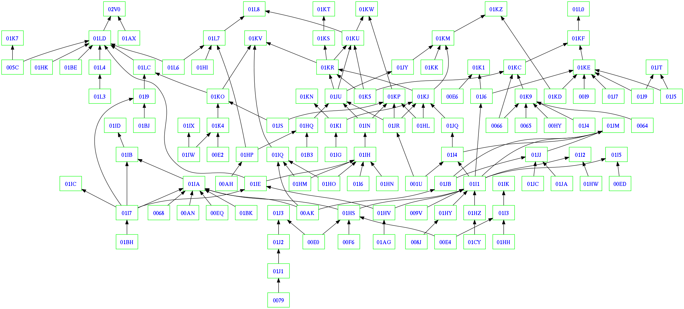