An easy way to think about priors on linear regression
Every time you add a prior to your multivariate linear regression it’s equivalent to changing the function you’re trying to minimize. It sometimes makes it easier to understand what’s going on when you think about it this way, and it only requires a bit of vector calculus. Of course it’s not the most sophisticated way of thinking of priors, which also have various bayesian interpretations with respect to the assumed distribution of the signals etc., but it’s handy to have more than one way to look at things.
Plain old vanilla linear regression
Let’s first start with your standard linear regression, where you don’t have a prior. Then you’re trying to find a “best-fit” vector of coefficients 


Here the various 
How do we find the minimum of that? First rewrite it in vector form, where we have a big column vector of all the different 


Now we appeal to an old calculus idea, namely that we can find the minimum of an upward-sloping function by locating where its derivative is zero.
Moreover, the derivative of 


Adding a prior on the variance, or penalizing large coefficients
There are various ways people go about adding a diagonal prior – and various ways people explain why they’re doing it. For the sake of simplicity I’ll use one “tuning parameter” for this prior, called 

In other words, we can think of trying to minimize the following more complicated sum:
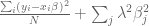
Here the 

When we minimize this, we are simultaneously trying to find a “good fit” in the sense of a linear regression, and trying to find that good fit with small coefficients, since the sum on the right grows larger as the coefficients get bigger. The extent to which we care more about the first goal or the second is just a question about how large 

How do we minimize that guy? Same idea, where we rewrite it in vector form first:

Again, we set the derivative to zero and ignore the factor of 2 to get:

Since 
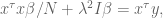

which of course can be rewritten as

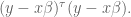
If you have a prior on the actual values of the coefficents of
Next I want to talk about a slightly fancier version of the same idea, namely when you have some idea of what you think the coefficients of 


We vectorize as

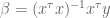
Again, we set the derivative to zero and ignore the factor of 2 to get:

so we can conclude:

which can be rewritten as


The first modification is Tichonov regularization.
LikeLike