mathbabe

Last night in Rachel Schutt’s Columbia Data Science course we had Matt Gattis come and talk to us about recommendation engines. Matt graduated from MIT in CS, worked at SiteAdvisor, and co-founded hunch as its CTO, which recently got acquired by eBay. Here’s what Matt had to say about his company:

Hunch

Hunch is a website that gives you recommendations of any kind. When we started out it worked like this: we’d ask you a bunch of questions (people seem to love answering questions), and then you could ask the engine questions like, what cell phone should I buy? or, where should I go on a trip? and it would give you advice. We use machine learning to learn and to give you better and better advice.

Later we expanded into more of an API where we crawled the web for data rather than asking people direct questions. We can also be used by third party to personalize content for a given site, a nice business proposition which led eBay to acquire us. My role there was doing the R&D for the underlying recommendation engine.

Matt has been building code since he was a kid, so he considers software engineering to be his strong suit. Hunch is a cross-domain experience so he doesn’t consider himself a domain expert in any focused way, except for recommendation systems themselves.

The best quote Matt gave us yesterday was this: “Forming a data team is kind of like planning a heist.” He meant that you need people with all sorts of skills, and that one person probably can’t do everything by herself. Think Ocean’s Eleven but sexier.

A real-world recommendation engine

You have users, and you have items to recommend. Each user and each item has a node to represent it. Generally users like certain items. We represent this as a bipartite graph. The edges are “preferences”. They could have weights: they could be positive, negative, or on a continuous scale (or discontinuous but many-valued like a star system). The implications of this choice can be heavy but we won’t get too into them today.

So you have all this training data in the form of preferences. Now you wanna predict other preferences. You can also have metadata on users (i.e. know they are male or female, etc.) or on items (a product for women).

For example, imagine users came to your website. You may know each user’s gender, age, whether they’re liberal or conservative, and their preferences for up to 3 items.

We represent a given user as a vector of features, sometimes including only their meta data, sometimes including only their preferences (which would lead to a sparse vector since you don’t know all their opinions) and sometimes including both, depending on what you’re doing with the vector.

Nearest Neighbor Algorithm?

Let’s review nearest neighbor algorithm (discussed here): if we want to predict whether a user A likes something, we just look at the user B closest to user A who has an opinion and we assume A’s opinion is the same as B’s.

To implement this you need a definition of a metric so you can measure distance. One example: Jaccard distance, i.e. the number of things preferences they have in common divided by the total number of things. Other examples: cosine similarity or euclidean distance. Note: you might get a different answer depending on which metric you choose.

What are some problems using nearest neighbors?

• There are too many dimensions, so the closest neighbors are too far away from each other. There are tons of features, moreover, that are highly correlated with each other. For example, you might imagine that as you get older you become more conservative. But then counting both age and politics would mean you’re double counting a single feature in some sense. This would lead to bad performance, because you’re using redundant information. So we need to build in an understanding of the correlation and project onto smaller dimensional space.
• Some features are more informative than others. Weighting features may therefore be helpful: maybe your age has nothing to do with your preference for item 1. Again you’d probably use something like covariances to choose your weights.
• If your vector (or matrix, if you put together the vectors) is too sparse, or you have lots of missing data, then most things are unknown and the Jaccard distance means nothing because there’s no overlap.
• There’s measurement (reporting) error: people may lie.
• There’s a calculation cost – computational complexity.
• Euclidean distance also has a scaling problem: age differences outweigh other differences if they’re reported as 0 (for don’t like) or 1 (for like). Essentially this means that raw euclidean distance doesn’t explicitly optimize.
• Also, old and young people might think one thing but middle-aged people something else. We seem to be assuming a linear relationship but it may not exist
• User preferences may also change over time, which falls outside the model. For example, at Ebay, they might be buying a printer, which makes them only want ink for a short time.
• Overfitting is also a problem. The one guy is closest, but it could be noise. How do you adjust for that? One idea is to use k-nearest neighbor, with say k=5.
• It’s also expensive to update the model as you add more data.

Matt says the biggest issues are overfitting and the “too many dimensions” problem. He’ll explain how he deals with them.

Going beyond nearest neighbor: machine learning/classification

In its most basic form, we’ve can model separately for each item using a linear regression. Denote by user ‘s preference for item (or attribute, if item is a metadata item). Say we want to model a given user’s preferences for a given item using only the 3 metadata properties of that user, which we assume are numeric. Then we can look for the best choice of as follows:

Remember, this model only works for one item. We need to build as many models as we have items. We know how to solve the above per item by linear algebra. Indeed one of the drawbacks is that we’re not using other items’ information at all to create the model for a given item.

This solves the “weighting of the features” problem we discussed above, but overfitting is still a problem, and it comes in the form of having huge coefficients when we don’t have enough data (i.e. not enough opinions on given items). We have a bayesian prior that these weights shouldn’t be too far out of whack, and we can implement this by adding a penalty term for really large coefficients.

This ends up being equivalent to adding a prior matrix to the covariance matrix. how do you choose lambda? Experimentally: use some data as your training set, evaluate how well you did using particular values of lambda, and adjust.

Important technical note: You can’t use this penalty term for large coefficients and assume the “weighting of the features” problem is still solved, because in fact you’re implicitly penalizing some coefficients more than others. The easiest way to get around this is to normalize your variables before entering them into the model, similar to how we did it in this earlier class.

The dimensionality problem

We still need to deal with this very large problem. We typically use both Principal Component Analysis (PCA) and Singular Value Decomposition (SVD).

To understand how this works, let’s talk about how we reduce dimensions and create “latent features” internally every day. For example, we invent concepts like “coolness” – but I can’t directly measure how cool someone is, like I could weigh them or something. Different people exhibit pattern of behavior which we internally label to our one dimension of “coolness”.

We let the machines do the work of figuring out what the important “latent features” are. We expect them to explain the variance in the answers to the various questions. The goal is to build a model which has a representation in a lower dimensional subspace which gathers “taste information” to generate recommendations.

SVD

Given a matrix compose it into three matrices:

Here is is is and is where is the number of users, is the number of items, and is the rank of

The rows of correspond to users, whereas has a row for each item. The square matrix is diagonal where each entry is a singular value, which measure the importance of each dimension. If we put them in decreasing order, which we do, then the dimensions are ordered by importance from highest to lowest. Every matrix has such a decomposition.

Important properties:

• The columns of and are orthogonal to each other.
• So we can order the columns by singular values.
• We can take lower rank approximation of X by throwing away part of In this way we might have much smaller than either or , and this is what we mean by compression.
• There is an important interpretation to the values in the matrices and For example, we can see, by using SVD, that “the most important latent feature” is often something like seeing if you’re a man or a woman.

[Question: did you use domain expertise to choose questions at Hunch? Answer: we tried to make them as fun as possible. Then, of course, we saw things needing to be asked which would be extremely informative, so we added those. In fact we found that we could ask merely 20 questions and then predict the rest of them with 80% accuracy. They were questions that you might imagine and some that surprised us, like competitive people v. uncompetitive people, introverted v. extroverted, thinking v. perceiving, etc., not unlike MBTI.]

More details on our encoding:

• Most of the time the questions are binary (yes/no).
• We create a separate variable for every variable.
• Comparison questions may be better at granular understanding, and get to revealed preferences, but we don’t use them.

Note if we have a rank matrix and we use the SVD above, we can take the approximation with only rows of the middle matrix so in other words we take the top most important latent features, and the corresponding rows of and and we get back something very close to

Note that the problem of sparsity or missing data is not fixed by the above SVD approach, nor is the computational complexity problem; SVD is expensive.

PCA

Now we’re still looking for and as above, but we don’t have anymore, so and we have a more general optimization problem. Specifically, we want to minimize:

Let me explain. We denote by the row of corresponding to user and similarly we denote by the row of corresponding to item Items can include meta-data information (so the age vectors of all the users will be a row in ).

Then the dot product is taken to mean the predicted value of user ‘s preference for item and we compare that to the actual preference . The set is just the set of all actual known preferences or meta-data attribution values.

So, we want to find the best choices of and which overall minimize the squared differences between prediction and observation on everything we actually know, and the idea is that if it’s really good on stuff we know, it will also be good on stuff we’re guessing.

Now we have a parameter, namely the number which is how may latent features we want to use. The matrix will have a row for each user and a column for each latent feature, and the matrix will have a row for each item and a column for each latent features.

How do we choose It’s typically about 100, since it’s more than 20 (we already know we had a pretty good grasp on someone if we ask them 20 questions) and it’s as much as we care to add before it’s computational too much work. Note the resulting latent features will be uncorrelated, since they are solving an efficiency problem (not a proof).

But how do we actually find and

Alternating Least Squares

This optimization doesn’t have a nice closed formula like ordinary least squares with one set of coefficients. Instead, we use an iterative algorithm like with gradient descent. As long as your problem is convex you’ll converge ok (i.e. you won’t find yourself at a local but not global maximum), and we will force our problem to be convex using regularization.

Algorithm:

• Pick a random
• Optimize while is fixed
• Optimize while is fixed
• Keep doing the above two steps until you’re not changing very much at all.

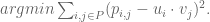
Example: Fix and update

The way we do this optimization is user by user. So for user we want to find

where is fixed. In other words, we just care about this user for now.

But wait a minute, this is the same as linear least squares, and has a closed form solution! In other words, set:

where is the subset of for which we have preferences coming from user Taking the inverse is easy since it’s which is small. And there aren’t that many preferences per user, so solving this many times is really not that hard. Overall we’ve got a do-able update for

When you fix U and optimize V, it’s analogous; you only ever have to consider the users that rated that movie, which may be pretty large, but you’re only ever inverting a  matrix.

Another cool thing: since each user is only dependent on their item’s preferences, we can parallelize this update of or We can run it on as many different machines as we want to make it fast.

There are lots of different versions of this. Sometimes you need to extend it to make it work in your particular case.

Note: as stated this is not actually convex, but similar to the regularization we did for least squares, we can add a penalty for large entries in and depending on some parameter which again translates to the same thing, i.e. adding a diagonal matrix to the covariance matrix, when you solve least squares. This makes the problem convex if is big enough.

You can add new users, new data, keep optimizing U and V. You can choose which users you think need more updating. Or if they have enough ratings, you can decide not to update the rest of them.

As with any machine learning model, you should perform cross-validation for this model – leave out a bit and see how you did. This is a way of testing overfitting problems.

Thought experiment – filter bubbles

What are the implications of using error minimization to predict preferences? How does presentation of recommendations affect the feedback collected?

For example, can we end up in local maxima with rich-get-richer effects? In other words, does showing certain items at the beginning “give them an unfair advantage” over other things? And so do certain things just get popular or not based on luck?

How do we correct for this?