hcssim | Search Results

Search Results

Keyword: ‘hcssim’

HCSSiM Workshop day 17

July 21, 2012 Cathy O'Neil, mathbabe Comments off

This is a continuation of this, where I take notes on my workshop at HCSSiM.

Magic Squares

First Elizabeth Campolongo talked about magic squares. First she exhibited a bunch, including these classic ones which I found here:

Then we noted that flipping or rotating a magic square gives you another one, and also that the trivial magic square with all “1”‘s should also count as a crappy kind of magic square.

Then, for 3-by-3 magic squares, Elizabeth showed that knowing 3 entries (say the lowest row) would give you everything. This is in part because if you add up all four “lines” going through the center, you get the center guy four times and everything else once, or in other words everything once and the center guy three times. But you can also add up all the horizontal lines to get everything once. The first sum is 4C, if C is the sum of any line, and the second sum is 3C, so subtracting we get that C is the the center three times, or the center is just C/3.

This means if you have the bottom row, you can also infer C and thus the center. Then once you have the bottom and the center you can infer the top, and then you can infer the two sides.

After convincing them of this, Elizabeth explained that the set of magic cubes was actually a vector space over the rational numbers, and since we’d exhibited 3 non-collinear ones and since we’d proved we can have at most 3 degrees of freedom for any magic square, we actually had a basis.

Finally, she showed them one of the “all prime magic squares”:

The one with the “17” in the corner of course. She exhibited this as a sum of the basis we had written down. It was very cool.

The game of Set

My man Max Levit then whipped out some Set cards and showed people how to play (most of them already knew). After assigning numbers mod 3 to each of the 4 dimensions, he noted that taking any two cards, you’d be able to define the third card uniquely so that all three form a set. Moreover, that third card is just the negative of the sum of the first two, or in other words the sum of all three cards in a set is the vector $(0, 0, 0, 0).$

Next Max started talking about how many cards you can have where they don’t form a set. He started in the case where you have only two dimensions (but you’re still working mod 3). There are clearly at most 4, with a short pigeon hole argument, and he exhibited 4 that work.

He moved on to 3 and 4 dimensions and showed you could lay down 9 in 3 and 20 in 4 dimensions without forming a set (picture from here), which one of our students eagerly demonstrated with actual cards:

Finally, Max talked about creating magic squares with sets, tying together his awesome lecture with Elizabeth’s. A magic square of sets is also generated by 3 non-collinear cards, and you get the rest from those three placed anywhere away from a line:

Probability functions on lattices

Josh Vekhter then talked about probability distributions as functions from posets of “event spaces” to the real line. So if you role a 6-sided die, for example, you can think of the event “it’s a 3, 4, or 6” as being above the event “it’s a 3”. He talked about a lattice as a poset where there’s always an “or” and an “and”, so there’s always a common ancestor and child for any two elements.

Then he talked about the question of whether that probability function distributes in the way it “should” with respect to “and” and “or”, and explained how it doesn’t in the case of the two slit experiment.

He related this lack of distribution law of the probability function to the concept of the convexity of the space of probability distributions (keeping in mind that we actually have a vector space of possibly probability functions on a given lattice, can we find “pure” probability distributions that always take the values of 0 or 1 and which form a kind of basis for the entire set?).

This is not my expertise and hopefully Josh will fill in some details in the coming days.

King Chicken

I took over here at the end and discussed some beautiful problems related to flocks of chickens and pecking orders, which can be found in this paper. It was particularly poignant for me to talk about this because my first exposure to these problems was my entrance exam to get into this math program in 1987, when I was 14.

Notetaking algorithm

Finally, I proved that the notetaking algorithm we started the workshop with 3 weeks before actually always works. I did this by first remarking that, as long as it really was a function from the people to the numbers, i.e. it never gets stuck in an infinite loop, then it’s a bijection for sure because it has an inverse.

To show you don’t get stuck in an infinite loop, consider it as a directed graph instead of an undirected graph, in which case you put down arrows on all the columns (and all the segments of columns) from the names to the numbers, since you always go down when you’re on a column.

For the pipes between columns, you can actually squint really hard and realize there are two directed arrows there, one from the top left to the lower right and the other from the top right to the lower left. You’ve now replaces the “T” connections with directed arrows, and if you do this to every pipe you’ve removed all of the “T” connections altogether. It now looks like a bowl of yummy spaghetti.

But that means there is no chance to fall into an infinite loop, since that would require a vertex. Note that after doing this you do get lots of spaghetti circles falling out of your diagram.

Categories: math education

HCSSiM Workshop day 16

July 20, 2012 Cathy O'Neil, mathbabe 2 comments

This is a continuation of this, where I take notes on my workshop at HCSSiM.

Two days ago Benji Fisher came to my workshop to talk about group laws on rational points of weird things in the plane. Here are his notes.

Degenerate Elliptic Curves in the plane

Conics in the plane

Pick $t \in \mathbb{R}$ . Consider the line $L_t$ given by $y = tx + t$ . Where does $L_t$ intersect the y-axis? Where does it intersect the unit circle, $x^2 + y^2 =1?$

Substitute $y = tx +t$ into the equation for the circle to get

$(1 + t^2) \, x^2 + (2 t^2) \, x + (t^2 - 1) = 0.$

After you do it the hard way, notice that you already know one root: $x = -1$ .

The sum of the roots is $-2 t^2 / (1 + t^2)$ and their product is $(t^2 - 1) / (t^2 + 1)$ . Either way, you get

$x = (1 - t^2) / (1 + t^2)$ .

From $y= t x + t$ you get $y = 2 t / (1 + t^2)$ .

Do not forget that if you are given $x$ and $y$ , then $t = y / (x + 1)$ .

This gives you a 1-1 correspondence between the points of the circle (conic) and the points of the $y$ -axis (including $\infty$ ). The formula for Pythagorean triples also falls out. So do the formulae for the tangent-of-the-half-angle substitution, which is useful when integrating rational functions of $\sin$ and $\cos$ : set $x = \cos(\theta),$ $y = \sin(\theta),$ and $t = \tan(\theta/2).$

There are several ways you can generalize this. You could project a sphere onto a plane. I want to consider replacing the circle with a cubic curve. The problem is that the expected number of intersections between a line and a cubic is 3, so you get a 2-to-1 correspondence in general. That is interesting, too, but for now I want to consider the cases where the curve has a double point and I choose lines through that point. Such lines should intersect the cube in one other point, giving a 1-1 correspondence between the curve (minus the singular point) and a line (minus a small number of points).

cubic with a cusp

Let $C$ be the curve defined by

$y^2 = x^3$ ,

which has a sharp corner at the origin. This type of singularity is called a cusp. Let $L_t$ denote the line through the origin and the point $(1,t)$ , which has slope $t$ .

Sketch the curve $C$ . Does Mathematica do a good job of this?
The line $L_t$ meets the curve $C$ at the origin and in one other point, $(x, y)$ . Find formulae for $x$ and $y$ in terms of $t$ and for $t$ in terms of $x$ and $y$ .
You almost get a digestion (bijection) between $C$ and the line $x = 1$ . What points do you have to omit from each in order to get a digestion?
Three points $(x_1, y_1), (x_2, y_2)$ , and $(x_3, y_3)$ on $C$ are collinear. What condition does this impose on the corresponding values of $t$ ?

The calculations are easier than for the circle: $x=t^2, y = t^3$ , and $t = y/x.$

You have to remove the point $(0, 0)$ from the curve and the point $(1, 0)$ from the line. Well, you do not have to remove them, but the formula for $t$ in terms of $x$ and $y$ is fishy if you do not. The point at infinity (the third point of intersection between the curve and the $y$ -axis) corresponds to itself.

The condition for colliniarity is

$\frac{y_3 - y_1}{x_3 - x_1} = \frac{y_2 - y_1}{x_2 - x_1}.$

Plug in the expressions in terms of the $t$ coordinates, chug away, and you should get

$t_1^{-1} + t_2^{-1} + t_3^{-1} = 0$ .

If we let $u = t^{-1}$ , then $u$ is the natural coordinate on the line $y=1$ . (Maybe I should use that line to start with instead of $x=1$ .)

cubic with a node

This problem deals with the curve $C$ defined by

$y^2 = x^3 + x^2$ ,

which intersects itself at the origin. This type of singularity is called a node. Let $L_t$ denote the line through the origin and the point $(1,t)$ , which has slope $t$ .

Sketch the curve $C$ . Does Mathematica do a good job of this?
The line $L_t$ meets the curve $C$ at the origin and in one other point, $(x, y$ ). Find formulae for $x$ and $y$ in terms of $t$ and for $t$ in terms of $x$ and $y$ .
You almost get a digestion (bijection) between $C$ and the line $x = 1$ . What points do you have to omit from each in order to get a digestion?
Three points $(x_1, y_1), (x_2, y_2)$ , and $(x_3, y_3)$ on $C$ are collinear. What condition does this impose on the corresponding values of $t$ ?

Once again, $t = y / x$ . The usual method gives $x = t^2 - 1$ and $y = t^3 - t$ . In order to get a 1-1 correspondence, you need to delete the singular point $(0,0)$ from the curve and the points $(1,1)$ and $(1,-1)$ from the line.

The lines through the origin with slope $\pm1$ are tangent to the curve. If you plug away, you should find that the condition for colliniarity is:

$t_1 t_2 + t_1 t_3 + t_2 t_3 + 1 = 0$ .

Remember our curve $C$ (not to be Maximum Confused with $\mathbb{C}$ )? It’s the one whose equation is $u^2 = x^3 + x^2.$ The condition for 3 points to be collinear on $C$ is:

$t_1 t_2 + t_2 t_3 + t_3 t_1 +1 = 0.$

Claim: in terms of $u = \frac{t-1}{t+1}$ , the condition is $u_1 u_2 u_3 = 1.$

(Hint: In terms of $u$ , $t = \frac{1+u}{1 - u}$ .)

If you start with the known equation and replace the $t$ ‘s with $u$ ‘s, it takes some work to get down to the condition $u_1 u_2 u_3 = 1$ .

If you start with the LHS of the desired equation, there is a shortcut:

$u_1 u_2 u_3 = \frac{t_1 - 1}{t_1 + 1} \cdot \frac{t_2 - 1}{t_2 + 1}$ $\cdot \frac{t_3-1}{t_3+1}$ .

But then we have

$u_1 u_2 u_3 = \frac{t_1 t_2 t_3 + t_1 + t_2 + t_3 - (t_1 t_2 + t_1 t_3 + t _2 t_3 + 1)}{t_1 t_2 t_3 + t_1 + t_2 + t_3 + (t_1 t_2 + t_2 t_3 + t_3 t_1 + 1)} = 1.$

Note that the change-of-variable formulae are fractional linear transformations. Geometrically, $t$ is the natural coordinate on the line $x=1$ and $u$ is the natural coordinate on the line $x + y = 1$ .

To get from one line to the other, just draw a line through the origin.

One interpretation of our results for the curves $y^2 = x^3$ , $y^2 = x^3 + x^2$ , is that it gives us a way to add points on the line $y = 1$ (with coordinate $t^{-1}$ ) and multiply points on the line $x + y = 1$ (with coordinate $u$ ) using just a straightedge, provided that we are allowed to draw lines through the point at infinity.

In other words, we are allowed to draw vertical lines. I will continue to refer to this as “straightedge only.” I forgot to mention: you need to have the curve provided as well. Explicitly, this is the rule. Given two points on the line, find the corresponding point on the curve. Draw a line through them. The third point of intersection with the curve will be the (additive or multiplicative) inverse of the desired sum. Draw a vertical line through this point: the second point of intersection (or the third, if you count the point at infinity as being the second) will be the desired sum/product.

More precisely, it is the point on the curve corresponding to the desired sum/product, so you have to draw one more line.

Another interpretation is that we get a troupe (or karafiol) structure on the points of the curve, excluding the singular point but including the point at infinity. The point at infinity is the identity element of the troupe (group). The construction is exactly the same as in the previous paragraph, except you leave off the parts about starting and ending on the line.

smooth cubic

Similarly, we get a troupe (group) structure on any smooth cubic curve. For example, consider the curve $E$ defined by

$E: y^2 = x^3 - x .$

Start with two points on the curve, say $P_1 = (x_1, y_1)$ and $P_2 = (x_2, y_2)$ . The equation for the line through these two points is $\frac{y - y_1}{x - x_1} = \frac{y_2 - y_1}{x_2 - x_1} = m .$ $

Solving for $y$ gives the equation $y = mx + b$ where $b = \frac{x_2 y_1 - x_1 y_2}{x_2 - x_1}.$

Plug this into the equation defining $R$ and you get, after a little algebra,

$x^3- m^2 x^2 - (2 m b + 1)x - b^2 = 0 .$

Luckily, we know how to solve the general cubic. (Just kidding! Coming back to what we did with the circle, we observe that $x_1$ and $x_2$ are two of the roots, so we can use either of the relations $x_1 + x_2 + x_3 = m^2$ or $x_1 x_2 x_3 = b^2$ .)

The result is:

$x_3 = m^2 - x_1 - x_2 = \frac{x_1^2 x_2 + x_1 x_2^2 - x_1 - x_2 - 2 y_1 y_2}{(x_1 - x_2)^3},$

where the final form comes from squaring $m$ and using the relations $y_1^2 = x_1^3 - x_1$ and $y_2^2 = x_2^3 - x_2$ .

At this point, a little patience (or a little computer-aided algebra) gives

$y_3 = \frac{(3 x_1 x_2^2 + x_2^3 - x_1 - 3 x_2) y_1 + (-x_1^3 - 3 x_1^2 x_2 + 3 x_1 + x_2) y_2}{(x_1 - x_2)^3}.$

Do not forget the final step: $P_3 = (x_3, y_3)$ is the third point of intersection, but to get the sum we need to draw a vertical line, or reflect in the $x$ -axis:

$P_1 \oplus P_2 = \overline{P_3} = (x_3, - y_3).$

Now, I give up. With a lot of machinery, I could exlpain why the group law is associative. (The identity, as I think I said above, is the point at infinity. Commutativity and inverses are clear.) What I can do with a different machine (Mathematica or some other computer-algebra system) is verify the associative law. I could also do it by hand, given a week, but I do not think I would learn anything from that exercise.

Some content on this page was disabled on December 15, 2019.

Categories: math education

HCSSiM Workshop day 15

July 19, 2012 Cathy O'Neil, mathbabe 2 comments

This is a continuation of this, where I take notes on my workshop at HCSSiM.

Aaron was visiting my class yesterday and talked about Sandpiles. Here are his notes:

Sandpiles: what they are

For fixed $m,n \ge 2$ , an $m \times n$ beach is a grid with some amount of sand in each spot. If there is too much sand in one place, it topples, sending one grain of sand to each of its neighbors (thereby losing 4 grains of sand). If this happens on an edge of the beach, one of the grains of sand falls off the edge and is gone forever. If it happens at a corner, 2 grains are lost. If there’s no toppling to do, the beach is stable. Here’s a 3-by-3 example I stole from here:

Do stable $m \times n$ beaches form a group?

Answer: well, you can add them together (pointwise) and then let that stabilize until you’ve got back to a stable beach (not trivial to prove this always settles! But it does). But is the sum well-defined?

In other words, if there is a cascade of toppling, does it matter what order things topple? Will you always reach the same stable beach regardless of how you topple?

Turns out the answer is yes, if you think about these grids as huge vectors and toppling as adding other 2-dimensional vectors with a ‘-4’ in one spot, a ‘1’ in each of the four spots neighboring that, and ‘0’ elsewhere. It inherits commutativity from addition in the integers.

Wait! Is there an identity? Yep, the beach with no sand; it doesn’t change anything when you add it.

Wait!! Are there inverses? Hmmmmm….

Lemma: There is no way to get back to all 0’s from any beach that has sand.
Proof. Imagine you could. Then the last topple would have to end up with no sand. But every topple adds sand to at least 2 sites (4 if the toppling happens in the center, 3 if on an edge, 2 if on a corner). Equivalently, nothing will topple unless there are at least 4 grains of sand total, and toppling never loses more than 2 grains, so you can never get down to 0.

Conclusion: there are no inverses; you cannot get back to the ‘0’ grid from anywhere. So it’s not a group.

Try again

Question: Are there beaches that you can get back to by adding sand?

There are: on a 2-by-2 beach, the ‘2’ grid (which means a 2 in every spot) plus itself is the ‘4’ grid, and that topples back to the ‘2’ grid if you topple every spot once. Also, the ‘2’ grid adds to the $(2, 0, 0, 2)$ grid and gets it back.

Wow, it seems like the ‘2’ grid is some kind of additive identity, at least for these two elements. But note that the ‘1’ grid plus the ‘2’ grid is the ‘3’ grid, which doesn’t topple back to the ‘1’ grid. So the ‘2’ grid doesn’t work as an identity for everything.

We need another definition.

Recurrent sandpiles

A stable beach C is recurrent if (i) it is stable, and (ii) given any beach A, there is a beach B such that C is the stabilization of A+B. We just write this C = A+B but we know that’s kind of cheating.

Alternative definition: a stable beach C is recurrent if (i) it is stable, and (ii) you can get to C by starting at the maximum ‘3’ grid, adding sand (call that part D), and toppling until you get something stable. C = ‘3’ + D.

It’s not hard to show these definitions are equivalent: if you have the first, let A = ‘3’. If you have the second, and if A is stable, write A + A’ = ‘3’, and we have B = A’ + D. Then convince yourself A doesn’t need to be stable.

Letting A=C we get a beach E so C = C+E, and E looks like an identity.

It turns out that if you have two recurrent beaches, then if you can get back to one using a beach E then you can get back to to the other using that same beach E (if you look for the identity for C + D, note that (C+D)+E = (C+E) + D = C+D; all recurrent beaches are of the form C+D so we’re done). Then that E is an identity element under beach addition for recurrent beaches.

Is the identity recurrent? Yes it is (why? this is hard and we won’t prove it). So you can also get from A to the identity, meaning there are inverses.

The recurrent beaches form a group!

What is the identity element? On a 2-by-2 beach it is the ‘2’ grid. The fact that it didn’t act as an identity on the ‘1’ grid was caused by the fact that the ‘1’ grid isn’t itself recurrent so isn’t considered to be inside this group.

Try to guess what it is on a 2-by-3 beach. Were you right? What is the order of the ‘2’ grid as a 2-by-3 beach?

Try to guess what the identity looks like on a 198-by-198 beach. Were you right? Here’s a picture of that:

We looked at some identities on other grids, and we watched an app generate one. You can play with this yourself. (Insert link).

The group of recurrent beaches is called the m-by-n sandpile group. I wanted to show it to the kids because I think it is a super cool example of a finite commutative group where it is hard to know what the identity element looks like.

You can do all sorts of weird things with sandpiles, like adding grains of sand randomly and seeing what happens. You can even model avalanches with this. There’s a sandpile applet you can go to and play with.

Categories: math education

HCSSiM 2012

July 18, 2012 Cathy O'Neil, mathbabe 18 comments

I was a senior staff member at the HCSSiM program in 2012, where I taught a workshop for the first half of the program, so 17 lectures, with my awesome junior staff Elizabeth Campolongo, Maxwell Levit, and Josh Vekhter.

I also gave a prime time theorem talk on the game of Nim.

I also wrote a bit about the tradition of Yellow Pig Day and the songs we sing every July 17th.

I also wrote a post about what is a proof and why mathematicians are trained to admit they’re wrong.

Here are the notes from the workshop:

Categories:

HCSSiM Workshop, day 14

July 18, 2012 Cathy O'Neil, mathbabe 7 comments

This is a continuation of this, where I take notes on my workshop at HCSSiM.

We switched it up a bit and I went to talk about Rubik’s Cubes in Benji Fisher’s classroom whilst Aaron Abrams taught in mine and Benji taught in Aaron’s. We did this so we could meet each other’s classes and because we each had a presentation that we thought all the classes might want to see.

In my class, besides what Aaron talked about (which I hope to blog about tomorrow), we talked about representing groups with generators and relations and we looked at how to create fractals on the complex plane using Mathematica.

Solving the Rubik’s Cube with group theory

First I talked about the position game, so ignoring orientation of the pieces. In other words, if all the pieces are in the correct position but are twisted or flipped, that’s ok.

Consider the group acting on the set which is the Rubik’s cube. We can fix the centers, and then this group is clearly generated by 90 degree clockwise turns on each of the 6 faces (clockwise when you look straight at the center of the face). It has a bunch of relations too, of course, including (for example) that the “front” move commutes with the “back” move and that any of these generators is trivial if you do it 4 times in a row.

Next we noted that the 8 corners always move to other corners on any of these moves, and that the 12 edges always move to edges. So we could further divide the “positions game” into an “edges game” and a “corners game.” Furthermore, because of this separation, any action can be realized as an element of the group

$S_8 \times S_{12}.$

But there’s more: any one of these generators is a 4-cycle on both edges and corners, which is odd in both cases, so so is a product of the generators. This means the group action actually lands inside

$A_8 \times A_{12} + B_8 \times B_{12},$

where I denote by $B_n$ the odd permutations of $S_n.$

Next I stated and proved that the 3-cycles generate $A_n$ , by writing any product of two transpositions as a product of two or three 3-cycles.

The reason that’s interesting is that, once I show that I can act by arbitrary 3-cycles on the edges or corners, this means I get that entire group up there of the form (even, even) or (odd, odd).

Next I demonstrated a 3-cycle on three “bad pieces” where one needs to go into the position of one of the other two. Namely:

Put two “bad” pieces on the top and one below, including the piece which is the destination of the third.
Do some move U which moves the third bad piece below to its position on the top without changing anything else.
Move the top so you decoy the new piece with the other bad piece on top. Call this decoy move V.
Undo the U move.
Undo the V move.

Seen from the perspective of the top, all that happens is that suddenly it has one piece in the right place (after U), then it gets rid of a piece it didn’t want anyway. From the perspective of the bottom, it sent up a piece it didn’t want to the top, then unmessed itself by taking back another piece from the top.

That’s a 3-cycle on the pieces, on the one hand (and a commutator on the basic moves), and we can perform it on any three corners or edges by first performing some move to get 2 out of the 3 pieces on the same face and the third not on that face. This is essentially acting by conjugation (and it’s still a commutator).

Moreover, the overall effect on the puzzle is that it took 3 pieces that were messed up and got at least 1 in the right spot.

The overall plan now is that you solve the corners puzzle, then the edges puzzle, and you’re done. Specifically, I get to the (even, even) situation by turning one face once if necessary, and then I can perform arbitrary 3-cycles to solve my problem. If I have fewer than three messed up corners (resp. edges), then I have either 0, 1, or 2 messed up corners (resp. edges). But I can’t have exactly 1, and exactly 2 would be odd, so I have 0.

That’s the position game, and I’ve given an algorithm to solve it (albeit not efficient!).

What about the orientations?

Shade the left and right side of a solved cube. Both the position (cubicle) and the piece of plastic (cubie) can be considered as shaded. Also shade a strip on the front and on the back, so we get the top and bottom edge of the front and back shaded.

Convince yourself that every edge and every corner position has exactly one shaded face.

When the cube is messed up, the shaded face of the position may not coincide with the shaded face of the cubie in that position. For edges it’s either right or wrong – assign each a value of 0 (if it’s right) or 1 (if it’s wrong). These can be considered orientation values modulo 2.

For corners, it can be wrong in two ways. The cubie’s shaded face could coincide with the position’s shaded face (give it a value 0), or it could be clockwise 120 degrees (value 1), or counterclockwise 120 degrees (value -1). These numbers are modulo 3.

Next, convince yourself that all of the generators of the group of actions on the rubik’s cube preserve the fact that the sum of the orientation numbers is 0, considered either mod 3 for the corners or mod 2 for the edges.

In particular, this means we can’t have exactly one edge flipped but everything in the right position. If you see this on a Rubik’s cube then someone took it apart and put it back together wrong.

However, you can twist one corner clockwise and another one counterclockwise, which means you can get any configuration of orientation numbers on the corners that satisfy that their sum is 0. Same with edges – it’s possible to flip two.

Finally, I exhibit how to do each of these basic orientation moves by 2 3-cycles. First I choose a pivot corner and perform a 3-cycle on those three corners, and then I do another 3-cycle, which uses the same 3 corners but is slightly different and results in everything being back in the right position but two corners twisted. I can do the same thing for edges, and I have thus totally solved the cube.

This method of 3-cycles is slow but it generalizes to all Rubik’s puzzles, so for example the 7 by 7 cube:

Or, with some work, something else like this:

p.s. I learned all of this when I was 15 from Mike Reid at HCSSiM 1987.

p.p.s. This was what we ate after singing our Yellow Pig Carols last night:

Categories: math education

HCSSiM Workshop, day 13

July 17, 2012 Cathy O'Neil, mathbabe 1 comment

This is a continuation of this, where I take notes on my workshop at HCSSiM.

Permutation notation

Using a tetrahedron as inspiration, we found the group of rotational symmetries as a subgroup of the permutation group $S_4.$ We then spent a lot of time discussing how to write good notation for permutations, coming up finally with the standard form but complaining about how multiplication is in a weird direction, stemming from the composition rule $(f \circ g)(x) = f(g(x)).$

Quadratic Reciprocity

Today we proved quadratic reciprocity, which totally rocks. In order to get there we needed three lemmas, which were essentially a bunch of different formulas for computing the Jacobi symbol.

The first was that, modulo $p$ we have:

$\left( \frac{a}{p} \right) \cong a^{(p-1)/2}.$

The second one was that we could write $\left( \frac{a}{p} \right)$ as -1 to the $n$ , where $n$ is the number of negative numbers you get when you write the numbers $a, 2a, 3a, \dots, \frac{p-1}{2} a$ modulo $p$ with a number of absolute value less than $p/2.$

In the third one we assume $a$ is odd (we deal with $a=2$ separately). We prove we can write $\left( \frac{a}{p} \right)$ as -1 to the $n$ , where $n$ is (also) the sum of the greatest integers $\left[ \frac{a j}{p} \right]$ for $j = 1, 2, 3, \dots, \frac{p-1}{2}.$

Each of these lemmas, in other words, gave us different ways to compute the symbol $\left( \frac{a}{p} \right)$ . They are each pretty easy to prove:

The first one uses the fact that if $a$ is not a square, then the product of all nonzero numbers mod $p$ can be paired up into $\frac{p-1}{2}$ pairs of different numbers whose product is $a$ , so we get altogether $a^{\frac{p-1}{2}},$ but on the other hand we already know by Wilson’s Theorem that that product is -1.

The second one just uses the fact that, ignoring negative signs, $a, 2a, 3a, \dots, \frac{p-1}{2} a$ is the same list as $j = 1, 2, 3, \dots, \frac{p-1}{2},$ but paying attention to negative signs we can take out an $a^{\frac{p-1}{2}}$ and also a $(-1)^n.$ Since we already know the first lemma we’re done.

The third lemma follows from repeatedly applying the division algorithm to $p$ and $aj$ , so writing

$\displaystyle{a j = p \cdot \left[\frac{aj}{p} \right] + r_j}$

for all $j= 1, 2, 3, \dots, \frac{p-1}{2}$ . We replace the remainders by the previous form of “small representatives” which we call $s_j$ modulo $p$ , making the remained positive or negative but smaller than $p/2;$ this replacement requires that we add $n p$ . We add all the division formulas up and realize that we only need to care about the parity of $n,$ so in other words we work modulo 2. It looks like this:

$a (1 + 2 + \dots + \frac{p-1}{2}) = \left( \left[\frac{a}{p} \right] + \left[\frac{2a}{p} \right]+ \dots + \left[\frac{\frac{p-1}{2} a}{p} \right] \right) p + s_1 + s_2 + \dots + s_{\frac{p-1}{2}} + n \cdot p.$

Since $a$ is odd, we can ignore it modulo 2. Since $p$ is odd same there. We get:

$1 + 2 + \dots + \frac{p-1}{2} = \left[\frac{a}{p} \right] + \left[\frac{2a}{p} \right]+ \dots + \left[\frac{\frac{p-1}{2} a}{p} \right] + s_1 + s_2 + \dots + s_{\frac{p-1}{2}} + n.$

Up to signs, $s_1 + s_2 + \dots + s_{\frac{p-1}{2}} = 1 + 2 + \dots + \frac{p-1}{2},$ so we can conclude our lemma.

Incidentally, using the formula above (before we ignore $p$ ) it’s also easy to see that $\left( \frac{2}{p} \right) = -1^{\frac{p^2-1}{8}}.$

Finally, we show that the sum $\left[\frac{a}{p} \right] + \left[\frac{2a}{p} \right]+ \dots + \left[\frac{\frac{p-1}{2} a}{p} \right]$ is just the number of lattice points in the region above the x-axis, to the left of the line $x = p/2,$ and below the line $y = \frac{a}{p} x.$

But, letting $a = q$ some other odd prime, we can do the same exact thing and we find that $\left[\frac{p}{q} \right] + \left[\frac{2p}{q} \right]+ \dots + \left[\frac{\frac{q-1}{2} p}{q} \right]$ is just the number of lattice points in the region above the x-axis, to the left of the line $x = q/2,$ and below the line $y = \frac{p}{q} x.$ Flipping the second triangle over the line $y = \frac{q}{p} x$ demonstrates that we have two halves of the rectangle with $\frac{p-1}{2} \frac{q-1}{2}$ lattice points. Here’s the picture for $p=19$ and $q = 7$ (ignore the dotted lines):

Therefore we’ve proved:

$\left( \frac{p}{q} \right) \left( \frac{q}{p} \right) = -1^{\frac{p-1}{2} \frac{q-1}{2}}.$

Alternating Group

We introduced cyclic notation, showing everything is a product of transpositions, then we introduced the sign function and showed that $e$ can only be written as a product of an even number of transpositions. This means the sign function is well defined, and it’s easy to see then that it’s a homomorphism, so we can define its kernel to be the alternating group.

Transformation of the Plane

We discussed rotations, shears, shrinks, reflections, and translations of the plane and demonstrated them in Mathematica using this.

Categories: math education

HCSSiM Workshop, day 12

July 15, 2012 Cathy O'Neil, mathbabe 8 comments

This is a continuation of this, where I take notes on my workshop at HCSSiM.

We originally defined $\mathbb{C}$ as $\mathbb{R}[x]/(x^2+1),$ and now we re-introduce it as the set of matrices of the form with the obvious map where $a + bi$ is sent to:

After we reminded people about matrix addition and multiplication, we showed this was an injective homomorphism under addition and also jived with the multiplication that we knew coming from $\mathbb{C}.$ Overall our lesson was not so different from this one.

Then we talked about actions on the plane including translations and scaling and showed that under the above map, “multiplication by $r e^{i \theta}$ ” or by its corresponding matrix gives us the same thing.

Platonic Solids

We went over the 5 platonic solids from yesterday- we’d proved it was impossible to have more than 5, and now it was time to show all 5 are actually possible! That’s when we whipped out Wayne Daniel’s “all five” puzzle:

We then introduced the concept of dual graph, and showed which platonic solids go to which under this map. We saw an example of a toy which flips from one platonic solid (cube) to its dual (octahedron) when you toss it in the air, the Hoberman Flip Out.

Here is it in between states:

Finally, we talked about symmetries of regular polyhedra and saw how we could embed an action into the group of symmetries on its vertices. So symmetries on tetrahedra is a subgroup of $S_4$ . It’s a lot easier to understand how to play with 4 numbers than to think about moving around a toy, so this is a good thing. Although it’s more fun to play with a toy.

Then one of our students, Milo, showed us how he projected a tiling of the plane onto the surface of a sphere using the language “processing“. Unbelievable.

After that we went to an origami workshop to construct yellow pigs as well as platonic solid type structures.

Categories: math education

HCSSiM Workshop, day 11

July 14, 2012 Cathy O'Neil, mathbabe 1 comment

This is a continuation of this, where I take notes on my workshop at HCSSiM.

Lagrange

We reminded people that a finite group is a finite set with an associative multiplication law “*”, and an identity and inverses with respect that law. A subgroup is a subset which is a group in its own right with the same multiplication law. Given a subgroup $H$ of a group $G,$ we defined the cosets of $H$ to be, for some $x \in G,$ of the form:

$x * H = \{y \in G | \exists h \in H, y = x *h \}.$

We proved that “being in the same coset as” is an equivalence relation and that each coset has the same size. Altogether the cosets form a partition of the group, so the size of the group is the product of the size of any coset and the number of cosets.

One of the students decided that you could form a group law on the set of cosets, inheriting the multiplication operation from $G.$ When it didn’t quite work out, he postulated that he could do it if the group is commutative. Pretty smart kid.

Primitive Roots modulo p

Next we spent more time than you’d think proving there’s a nonzero number $a$ modulo $p$ whose powers generate all of the nonzero elements modulo $p.$ In other words, that there is an isomorphism

$\mathbb{Z}/p\mathbb{Z} -$ $\{0\} \rightarrow \mathbb{Z}/(p -1) \mathbb{Z}.$

The left group is a group under multiplication, and the right one is a group under addition, which means this can be seen as a kind of logarithm in finite groups. Indeed an element $x$ on the left is mapped to that power $i$ of $a$ such that $a^i = x.$ So it’s very much like a logarithm.

To prove such an $a$ exists, we actually show that $\phi(p-1)$ such roots exist, and that in fact there are $\phi(d) d$ th roots of unity for any $d$ which divides $p-1.$ Another case where it helps to prove something harder than what you actually want.

To do that, we have a few lemmas. First, that there are at most $n$ roots to a degree $n$ polynomial modulo $p$ unless it’s the “zero” polynomial. Second, that if there’s a polynomial which achieves this maximum, it must divide the “Fermat’s Little Theorem” polynomial $X^p - X.$ These two lemmas aren’t hard.

Next we proved that there are at most $\phi(d)$ primitive $d$ th roots of unity for any $d,$ by showing that, if we had one, then we’d take certain powers to get all $\phi(d)$ of them, and then if we hadn’t counted one then we’d be able to produce too many roots of the polynomial $X^d -1.$

Finally, we wrote out boxes labeled with the divisors of $p-1$ and we labeled $p-1$ balls the non-zero numbers mod $p.$ We put a ball with label $b$ into the box with its order (the smallest positive number $i$ so that $b^i =1$ ). Since there are at most $\phi(d)$ in each box, and since we need to put every ball in some box, there must be exactly $\phi(d)$ balls in each box since we proved a few days ago that:

$p-1 = \sum_{d | (p-1)} \phi(d).$

Platonic Solids

Riffing on our proof of Euler’s formula for planar graphs, we convinced the kids that we could just as well consider a graph to be on a sphere, using a stereographic projection.

Then, using graphs on spheres as guides, we looked at how many examples we could come up with for a regular polytope, where each face has the same number of edges and each vertex has the same number of edges leaving it. We came up with the five platonic solids.

Categories: math education

HCSSiM Workshop day 10

July 13, 2012 Cathy O'Neil, mathbabe 2 comments

This is a continuation of this, where I take notes on my workshop at HCSSiM.

Quadratic equations modulo p

We looked at the general quadratic equation $a x^2 + b x + c$ modulo an odd prime $p$ (assume $a \not \cong 0 \; \; (mod \; p)$ ) and asked when it has roots. We eventually found the solution to be similar to the one we recognize over the reals, except you need to multiply by $(2 a)^{-1}$ instead of dividing by $2a$ . In particular, we achieved the goal, which was to reduce this general form to a question of when a certain thing (in this case $b^2 - 4ac$ ) is a square modulo $p$ , in preparation for quadratic reciprocity.

We then defined the Jacobi symbol 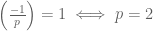$\left( \frac{a}{p} \right)$ and proved that $\left( \frac{-1}{p} \right) = 1 \iff p=2$ or $p \cong 1 \; \; (mod \; 4)$ .

Cantor

We then reviewed some things we’d been talking about in terms of counting and cardinality, we defined the $\leq$ notation for sets: we define $X \leq Y$ to mean “exists an injection from $X$ to $Y$ “. We showed it is a partial ordering using Cantor-Schroeder-Bernstein.

Then we used Cantor’s argument to show the power set of a set always has strictly bigger cardinality than the set.

Euler and planar graphs

At this point the CSO (Chief Silliness Officer) Josh Vekhter took over class and described a way of assessing risk for bank robbers. You draw out a map of a bank as a graph with vertices in the corners and edges as walls. It can look like a tree, he said, but it would be a pretty crappy bank. But no judgment. He decided that, from the perspective of a bank robber, corners are good (more places to hide), rooms are good (more places for money to be stashed) but walls are bad (more things you need to break through to get money.

With this system, and assigning a -1 to every wall and a 1 to every corner or room, the overall risk of a bank’s map consistently looks like 2. He proved this is always true using induction on the number of rooms.

Categories: math education

HCSSiM Workshop day 9

July 12, 2012 Cathy O'Neil, mathbabe 4 comments

A continuation of this, where I take notes on my workshop at HCSSiM.

First we had a few proofs from the previous night’s problem set, including a proof of Hall’s Marriage Problem using Dilworth’s Theorem.

Counting stuff

We then proved an uncountable set union a countable set is uncountable, with the help of Lior’s comment from yesterday.

Then we proved the Cantor-Schroeder-Bernstein Theorem, which states that if you have two injective maps $f$ and $g$ in the opposite directions: $f:X \rightarrow Y$ and $g:Y \rightarrow X,$ then you can construct a bijection between $X$ and $Y$ , and in particular the two sets will have the same cardinality. It’s not that hard – consider the orbits of points in X and Y under repeated applications of the two injective maps $f,g$ , and if possible, by pulling back by $f^{-1}$ and $g^{-1}.$

It doesn’t take much thinking to convince yourself that these orbits come in three forms: an infinite list in both directions, a finite loop, or an infinite forward path but a finite backwards path, where at some point you can’t pull back any more. In the last case you could get “stuck” in either $X$ or $Y.$ Since the orbits form a partition of all of the points, you can independently decide how to define the bijection depending on what that orbit looks like. Namely, it takes an element $x$ in $X$ to $f(x)$ unless it’s an orbit that gets going backwards in $Y,$ in which case you take $x$ to $g^{-1}(x).$

Now that I think of it, I’m pretty sure this proof uses the axiom of choice, and according to the wikipage on this theorem it doesn’t need to, but I don’t know a proof which avoids it. The truth is I can never tell. Please explain to me if you can, how you can verify if you’re using the axiom of choice in an argument where you make infinitely many decisions.

Homomorphisms

We defined a homomorphism of groups and wrote it in both additive and multiplicative notation, because it turns out some of the students were getting confused. We proved very basic properties that follow such as the fact that the identity element goes to the identity element under a homomorphism, and the image of the inverse of an element is the inverse of the image. We ended by asking them to consider the set of homomorphisms between a cyclic group of 6 elements and itself, or between a cyclic group of 6 elements to a cyclic group of 7 elements.

Fermat and Wilson

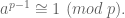
Next we whipped out some theorems modulo a prime $p.$ We looked at the action defined on numbers mod 17 when you multiply them by 3, and noticed it just scrambles the non-zero ones up (and of course sends 0 to 0). We proved that this is true in general. But this means that the product of all the non-zero numbers mod p is the same if we pre-multiply by any $a$ , which means that product is equal to itself times $a^{p-1},$ and since it’s invertible that means $a^{p-1} \cong 1 \, \, (mod \; p).$ That’s just a hop skip and jump away from Fermat’s Little Theorem, which states that $a^{p} \cong a \, \, (mod \; p)$ for every number $a$ .

Next, we wondered, what was that product of all those non-zero numbers mod $p$ ? It turns out that each of those nonzero guys is invertible, so if you pair each up with its inverse their contribution to the product is just 1, and the leftovers are just the guys who are their own inverse, which is only 1 or -1 (which we proved, and which is most definitely not true modulo 8). So the whole product is -1. That’s Wilson’s Theorem, but we called it Wilevson’s Theorem since Lev came up with the argument.

Categories: math education

HCSSiM Workshop day 8

July 11, 2012 Cathy O'Neil, mathbabe 2 comments

A continuation of this, where I take notes on my workshop at HCSSiM.

We first saw presentations from the students from last night’s problem set. One was a four line proof that the last two digits of $17^{2012}$ are 61. The other was a beautiful proof that the only real numbers that have more than one decimal representation are rationals of the form $a/10^k$ for some integer $k.$

Dillworth’s Theorem Revisited

After going over examples of chains and antichains, and making sure we knew that there must be at least as many chains as there are elements in an anti-chains if we want the chains to cover our set, we set up a proof by induction on the number of elements in our set. The base case is easy (one element, one chain, one element in a maximal anti-chain) and then to reduce to a smaller case we remove any maximal element $m$ . Note this just means there’s nothing above it. But now the inductive hypothesis holds, and we cover the remaining set with chains $C_1, C_2, \dots, C_k$ and moreover we define $a_i \in C_i$ to be the largest element in $C_i$ such that it is contained in some maximal anti-chain.

We then stated two lemmas. The first is that any maximal anti-chain must have a unique element in each chain $C_i$, and the second is that, after defining the elements $a_i$ as above, they form a maximal anti-chain. We treat these lemmas as black boxes for the proof (the first we did yesterday, the second is on problem set tonight).

Now we put back the removed point $m.$ There are two cases, either $m$ is incomparable to any of the $a_i$ ‘s or it is comparable to at least one of them.

In the first case, we have an anti-chain of size $k+1,$ namely the $a_i$ ‘s plus $m$ , and we can form a $(k+1)$ st chain consisting of just $m$ itself.

In the second case, $m$ is comparable to some $a_i.$ Since $m$ is maximal, and since $a_i$ is maximal in its chain $C_i$ with respect to being in a maximal antichain, we can form a new chain which is just the same thing as $C_i$ for $a_i$ and below, and goes straight up to $m$ from $a_i.$ Note we may be missing some stuff that used to be above $a_i$ in $C_i.$ But that doesn’t matter, because if we remove this new chain, we see that the maximal anti-chains leftover is only of size $k-1,$ so by Strong Induction we can cover it with $k-1$ chains, and then bring back this chain to get an overall covering with $k$ chains.

Dihedral Groups

After reviewing the formal definition of a Karafiol (group), we used rotations and flips of a folder and then of a regular 5-gon to come up with a non-commutative group. We defined a subgroup and explored the different subgroups of the dihedral group as well as other examples we’d seen coming from modular arithmetic.

Euler’s Totient function

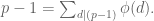
We introduced the number of positive integers less than $n$ relatively prime to $n$ as a function of $n$ called $\phi(n)$ and wrote out a table up to 17. We observed that $\phi(p) = p-1$ and that, from the Chinese Remainder Theorem, we also could infer that for $gcd(m, n) = 1$ we have $\phi(mn) = \phi(m) \phi(n).$ Writing out a prime factorization for $n = \prod_i p_i^{a_i}$ we realized we’d have a formula for $\phi(n)$ if we just knew $\phi(p^a)$ for any prime $p$ and any positive $a.$ We wrote out a picture and decided $\phi(p^a) = p^a - p^{a-1}.$

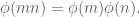
We ended by proving Euler’s formula by induction on the number of distinct prime factors:

$\sum_{d | n} \phi(d) = n.$

Categories: math education

HCSSiM Workshop day 7

July 10, 2012 Cathy O'Neil, mathbabe 4 comments

A continuation of this, where I take notes on my workshop at HCSSiM.

The real numbers are uncountable

Today we used Cantor’s diagonal argument to prove that the real numbers aren’t countable. Namely, we assumed they were, and that we had a bijection $f: \mathbb{N} \rightarrow \mathbb{R}$ and then proved it didn’t contain the real number $YP,$ whose $i$ th digit we defined to be 1 if the $i$ th digit of $f(i)$ is 7, and 7 otherwise. One of our students pointed out that there are some numbers that have more than one decimal expansion, so the general argument that a certain decimal expansion isn’t in the list isn’t a total proof. But we decided that we’d be able to prove on homework that the only numbers that have more than one representative in decimal expansions are rational with their denominators divisible only by 2 and 5, which is not the case for the number YP we’d been talking about.

Then we wanted to show that $\mathbb{R}$ has the same cardinality as $\mathbb{R}\times\mathbb{R}.$ We tried to use a “splicing argument” where we create a new decimal expansion out of two decimal expansions (where the odd digits correspond to the first and the even to the second), but then we decided this map isn’t well defined, since we still have this “overlap” problem where 0.999… = 1 but the pair $(0, 0.999...)$ doesn’t get mapped by the splicing map to the same decimal expansion as the pair $(0, 1).$

So then we decided to instead consider the set of decimal expansions, which is a bit bigger than the reals, and there the splicing map works. We reduced it to this case and are leaving it to homework to prove that the set of decimal expansions has the same cardinality as the reals. Although I don’t actually know how to do this without Cantor-Schroder-Bernstein, which we haven’t proven yet.

The Chinese Remainder Theorem

We stated and proved the Chinese (Llama) Remainder Theorem. It was a nice example of a constructive proof that assumes it’s possible and then, when you follow your nose, it’s possible to completely characterize what the solution must look like, and then it falls out. We showed it described a bijection of sets $\mathbb{Z}/\prod_i n_i \mathbb{Z} \rightarrow \prod_i \mathbb{Z}/n_i \mathbb{Z}.$ We haven’t talked about homomorphisms of groups yet though so we can’t prove it’s an isomorphism of groups.

Dilworth’s Theorem on chains and anti-chains in posets

We started the proof of Dilworth’s Theorem but didn’t finish yet (to be continued tomorrow). Turns out that this problem is really hard and that, moreover, there are lots of ways to convince yourself it’s true but be wrong about. The inductive proof in wikipedia, for example, is incomplete, but can be extended to a complete proof.

As an example, try to cover the following poset on the power set of five letters with 10 chains:

In particular you can see we solve a matching problem on the way, between subsets of size two and subsets of size 3 in the set of five letters, which isn’t the normal “take the complement” match, but rather is an inclusion of one in the other. I’m still wondering if there’s a more direct way to do this.

Categories: math education

HCSSiM Workshop day 6

July 8, 2012 Cathy O'Neil, mathbabe 4 comments

A continuation of this, where I take notes on my workshop at HCSSiM.

What is a group

We talked about sets with addition laws and what that really means. We noted that associativity seems to be a common condition and that some weird operations aren’t associative. Example: define $a*b$ for a pair of integers $(a,b)$ to be the sum $a + b^2.$ Then we have:

$(1*1)*1 = 2*1 = 3$ but $1*(1*1) = 1*2 = 5$ .

We decided those things would make them crappy generalized addition operators. We ended up by defining what a group is, although we call it a “Karafiol” so that when our final senior staff member P.J. Karafiol arrives in a couple of weeks he will already be famous.

We showed that $\mathbb{Z}/n \mathbb{Z}$ is a Karafiol and that, if you remove all of the congruence classes with numbers that aren’t relatively prime to $n,$ you can also turn $\mathbb{Z}/n \mathbb{Z}$ into a group under multiplication. I was happy to hear them challenge us on whether that would be closed under multiplication. The kids proved everything, we were just mediating. They are awesome.

Graphs

We had already talked about graphs (“Visual Representations”) as defined by vertices and edges. Today we talked about being able to put vertices in different groups depending on how the edges go between groups, so we ended up talking about bipartite and tripartite graphs. We ended up being convinced that the complete bipartite graph on 6 vertices (so 3 on each side) is not planar. But we haven’t proven it yet.

Special Lecture

Saturday morning we have only two hours of normal class, instead of 4, and we have a special event for the late morning. Yesterday Johan was visiting so he talked to them about the projective plane over a finite field, and how every line has the same number of points. He talked to them a bit about his REU at Columbia and his Stacks Project and the graph of theorems t-shirt that he wore to the talk. I think it’s cool to show the students this kind of thing because they are the next generation of mathematicians and it’s great to get them into online collaborative math as soon as possible. They were impressed that the Stack Project is more than 3000 pages.

Categories: math education

HCSSiM Workshop day 5

July 7, 2012 Cathy O'Neil, mathbabe 2 comments

A continuation of this, where I take notes on my workshop at HCSSiM.

Modular arithmetic

We examined finite sets with addition laws and asked whether they were the “same”, which for now meant their addition table looked the same except for relabeling. Of course we’d need the two sets to have the same size, so we compared $\mathbb{Z}/2\mathbb{Z} \times \mathbb{Z}/2\mathbb{Z}$ and $\mathbb{Z}/4\mathbb{Z}.$ We decided they weren’t the same, but then when we did it for $\mathbb{Z}/3\mathbb{Z} \times \mathbb{Z}/4\mathbb{Z}$ and $\mathbb{Z}/12 \mathbb{Z},$ and decided those were. We eventually decided it worked the second time because the moduli are relatively prime.

We essentially finished by proving the base case of the Chinese Remainder Theorem for two moduli, which for some ridiculous reason we are calling the Llama Remainder Theorem. Actually the reason is that one of the junior staff (Josh Vekhter) declared my lecture to be insufficiently silly (he designated himself the “Chief Silliness Officer”) and he came up with a story about a llama herder named Lou who kept track of his llamas by putting them first in groups of n and then in groups of m and in both cases only keeping track of the remaining left-over llamas. And then he died and his sons were in a fight over whether someone stole some llamas and someone had to be called in to arbitrate. Plus the answer is only well-defined up to a multiple of mn, but we decided that someone in town would have noticed if an extra mn llamas had been stolen.

Cardinality

After briefly discussing finite sets and their sizes, we defined two sets to have the same cardinality if there’s a bijection from one to the other. We showed this condition is reflexive, symmetric, and transitive.

Then we stopped over at the Hilbert Hotel, where a rather silly and grumpy hotel manager at first refused to let us into his hotel even though he had infinitely many rooms, because he said all his rooms were full. At first when we wanted to just add us, so a finite number of people, we simply told people to move down a few times and all was well. Then it got more complicated, when we had an infinite bus of people wanting to get into the hotel, but we solved that as well by forcing everyone to move to the hotel room number which was double their first. Then finally we figured out how to accommodate an infinite number of infinite buses.

We decided we’d proved that $\mathbb{N} \times \mathbb{N}$ has the same cardinality as $\mathbb{N}$ itself. We generalized to $\mathbb{Q}$ having the same cardinality as $\mathbb{N},$ and we decided to call sets like that “lodgeable,” since they were reminiscent of Hilbert’s Hotel.

We ended by asking whether the real numbers is lodgeable.

Complex Geometry

Here’s a motivating problem: you have an irregular hexagon inside a circle, where the alternate sides are the length of the radius. Prove the midpoints of those sides forms an equilateral triangle.

It will turn out that the circle is irrelevant, and that it’s easier to prove this if you actually Circle is entirely prove something harder.

We then explored the idea of size in the complex plane, and the operation of conjugation as reflection through the real line. Using this incredibly simple idea, plus the triangle inequality, we can prove that the polynomial

$3z^{17} + 2iz^{12} - (1+3i)z^{10} + .017z^{5} - 17$

has no roots inside the unit circle.

Going back to the motivating problem. Take three arbitrary points A, B, C on the complex plane (i.e. three complex numbers), and a fourth point we will assume is at the origin. Now rotate those three points 60 degrees counterclockwise with respect to the origin – this is equivalent to multiplying the original complex numbers by $e^{\frac{i \pi}{6}}.$ Call these new points A’, B’, C’. Show that the midpoints of the three lines AB’, BC’, and CA’ form an equilateral triangle, and that this result also is sufficient to prove the motivating problem.

Categories: math education

HCSSiM Workshop day 4

July 6, 2012 Cathy O'Neil, mathbabe 2 comments

A continuation of this, where I take notes on my workshop at HCSSiM.

As usual, we started with the students showing us solutions to their problem sets. Today one of them showed a sharp lower bound on the Fibonacci numbers, although he hadn’t proved it was sharp.

Arithmetic modulo n

Then we talked more about how we can talk about addition, and now also multiplication, with a finite set of symbols $\{0, 1, 2, \dots n-1\}$ . Then we wrote out the multiplication tables for $n = 6$ and $n = 7.$ The students noticed and proved that there is a multiplicative inverse for $a$ modulo $n$ if and only if $gcd(a, n) = 1,$ using what we did yesterday with the Edwinian Algorithm and the way we turned it around to express gcd’s as linear combinations. We defined some notation and the natural map:

$\mathbb{Z} \rightarrow \mathbb{Z}/n\mathbb{Z}.$

Finally, we wrote down the subsets of $\mathbb{Z}$ which map to each element of $\mathbb{Z}/n\mathbb{Z}.$

Posets and graphs

We went back to the idea of a partial ordering, and came up with a bunch of examples (including the set of integers under “divides evenly into”). We talked for a while about how to represent partial orderings, and finally settled on a graph. We talked a bit about poset chains and antichains, and then we formally defined a graph (we voted and decided to call it a “visual representation”).

The complex plane

The founder and director of the program is David Kelly. The program has been going for 40 years now and for maybe the first time ever Kelly himself isn’t teaching a workshop, so I’ve invited him to do some guest lectures in my workshop on complex geometry. It’s always a treat to watch him teach.

Kelly came in and built on the idea of “modding out by an integer” by definine $\mathbb{R}[x]/(x^2 +1),$ which he described as “modding out by a polynomial”. He asked the students to investigate this idea and they eventually discovered that if $x^2 +1 = 0,$ it also must be true that $x^2 = -1,$ which allowed them to write every polynomial with as a linear combination of 1 and $x,$ so as $a + bx$ . Then they thought about the addition law and multiplication law and decided they had the complex plane. So we decided to start calling $x$ the symbol “ $i$ “.

We then defined $e^{i \theta}$ to be the point on the unit circle $cos(\theta) + i sin(\theta),$ discarding once and forever the notation $cis(\theta)$ (we justified this definition in last night’s problem set). We showed we could recover useful trigonometric identities that way (I skipped trigonometry myself and this is the only way I ever knew how to derive those identities) and that we could alternatively write any point on the complex plane in polar coordinates, so as $r e^{i \theta}$ . Finally, we noted that if we multiply anything by the number $r e^{i \theta}$ , we end up stretching it by $r$ and rotating it by $\theta$ .

We heard a funny story Kelly told us about taking a test to get his pilot’s license. He was given 30 minutes and lots of suggestions once to compute a heading which involved a calculation in polar coordinates. Since he was a mathematician he was too proud to accept the props they offered him, and finished with 29 minutes to spare. Once aloft though he quickly realized his calculation simply couldn’t be correct, but fudged the test by eyeballing it and following a highway. Turns out that pilots use due north as the axis along which the angle is zero, and then they go clockwise from there. I’m not sure what the moral of the story is, but it’s something like, “don’t be arrogant unless it’s a clear day and you have a backup plan.”

Categories: math education

HCSSiM Workshop day 3

July 5, 2012 Cathy O'Neil, mathbabe 1 comment

A continuation of this, where I take notes on my workshop at HCSSiM.

Equivalence Relations and Partial Orderings

After going over many proofs of the geometry problem from last night’s problem set, I corrected the mistake in the “antisymmetric” property and we went through plenty of examples of equivalence relations and partial orderings. We ended with linear orderings, the real numbers, and the less than or equal relation.

Adding modulo n

Next we went back to the idea of maps $f: X \times X \rightarrow X$ and got the kids to come up with a whole bunch of examples for $X = \mathbb{Z},$ such as $f(a, b) = \lceil \frac{a}{2 \dot b +1} \rceil$ . We eventually got them to come up with stupider examples like $(a, b) \mapsto a$ and $(a, b) \mapsto a+b.$ Then we switched it up to the finite set $[n] = \{1, 2, 3, \dots, n\}$ and got them to generalize addition. Since $n$ really started to look like an identity element under this operation, we decided to define notation for the set $\{0, 1, 2, \dots, n-1\},$ which is like $[n]$ but on its side.

Pigs-in-hole Principle

We introduced the pigeonhole principle (but since our camp mascot is a yellow, pig, we call it pigs-in-hole). We actually defined the slightly more general idea that, if you have $n$ holes and $k$ pigs which need to get put into holes, at least one of the $n$ holes to contain at least $\lceil k/n \rceil$ pigs. With that we proved that at least 2 people in New York City have the same number of hairs on their head, that five points in a 1 by 1 square are withing distance $\sqrt{2}/2$ of each other, that in a group of $n$ people at least two people will have had the same number of handshakes, and others.

Greatest Common Divisor

We asked the kids what the greatest common divisor of $a$ and $b$ is (denoted $gcd(a, b)$ ) and how to compute it. We spent a long time chasing down rabbit holes and proving other things that didn’t help us find the greatest common divisor but were true. For example, we showed that if you divide $a$ and $b$ by their greatest common divisor, you end up with numbers that are relatively prime. We even showed there are representations of $a$ and $b$ as products of primes, but since we couldn’t yet prove those were unique representations, we could use that to come up with a way to find the “common primes.”

Eventually we thought of a trick to reduce the problem, namely the division algorithm. Actually Edwin thought of the trick, and it eventually became the Edwinian Algorithm (not like it’s usually called, namely the Euclidean Algorithm). Edwin observed that $gcd(a, b) = gcd(a - bq, b)$ when you write $a = bq + r$ for $0 \leq r <b.$

Once we had the Edwinian Algorithm, we realized we could go backwards and express $gcd(a, b)$ as a linear combination of $a$ and $b$ , and we used that to prove a very important property of primes, namely that if $p$ is a prime and $p | ab$ then either $p|a$ or $p|b$ or both. This allowed us to show that the prime factorizations we’d found before for $a$ and $b$ were in fact unique up to relabeling, which we left for homework.

So it turns out I’m not going to be able to make the homeworks public, but we had an awesome problem set with lots of pigeon hole problems and Edwinian Algorithm problems. We asked them to decide which approach to calculating $gcd(a,b)$ is faster, through the Edwinian Algorithm or via prime factorizations.

Categories: math education

HCSSiM Workshop day 2

July 4, 2012 Cathy O'Neil, mathbabe 3 comments

A continuation of this, where I take notes on my workshop at HCSSiM.

The watermelon cutting problem revisited

We prove that the maximum number of pieces of watermelon you can cut with $n$ slices, assuming a watermelon of dimension $d$ , denoted by $M_d(n),$ is given by:

$\sum_{k=0}^d \binom{n}{k}.$

First we proved it with a combinatorial argument, then with induction. I decided the first one is better because you figure out the answer as you go, whereas the induction route requires that you already know the formula. They both require you to use the recursion relation we talked about yesterday, and the first one involved writing a 2-d chart and showing how to unpack the value of $M_d(n),$ using the recurrence relation, into paths going up to the top row consisting of all ones, and then the question becomes, “how many ways can you get to the top row?” and of course the answer is something like $\binom{n}{k}$ , where you go up $n$ times and left $k$ times.

All pigs are yellow

Next we proved, using induction, that all pigs are the same color, and then we exhibited a yellow pig so a corollary was that all pigs are yellow. The base case is that a single pig is the same color as itself, and then assuming we have n pigs of the same color, we get to the statement that n+1 pigs are all the same color by first putting one pig in the barn, and then some other pig in the barn, and the leftover pigs are the same color as each of those so they’re all the same color.

This argument, of course, doesn’t work when you’re moving from “1 pig” to “2 pigs” and exhibits how careful you have to be with working through enough base cases so that your inductive step actually applies.

Strong Induction

We then went to using the Principle of Strong Induction (after showing that there’s no Principle of Induction over the real numbers). We proved that all numbers can be written as the sum of powers of 2, that the Fibonacci numbers grow exponentially, that every positive integer at least 2 is divisible by a prime, and that every planar polygon can be diagonalized using strong induction.

Notation

Incidentally, instead of “Strong Induction” the students voted to call it “Thor Induction”, and instead of the standard end-of-proof symbol, which is a box with an “x” inside, we voted to use the symbol “(see next page)”. They had lots of fun with that one. As a corollary, they decided that if they wanted someone to actually see the next page, they’d use the “Q.E.D.” symbol.

Cross product of Sets

Finally, we talked about the notation $X \times Y,$ which denotes the cross product of sets, and made a bunch of examples, mostly of the form $X \times X,$ specifically when $X = \mathbb{R}$ and $\mathbb{Z},$ which we then drew as the plane and the lattice points. We ended by showing an injection from $\mathbb{Z}$ into the lattice points, which incidentally showed that $\mathbb{Z}$ and $\mathbb{Z} \times \mathbb{Z}$ have the same cardinality, which we didn’t really define but we will.

Categories: math education

HCSSiM workshop day 1

July 3, 2012 Cathy O'Neil, mathbabe 17 comments

So I’ve decided to try to explain what we’re doing in class here at mathcamp. This is both for your benefit and mine, since this way I won’t have to find my notes next time I do this.

Notetakers

We started the math, after intros, by assigning note-takers. In one row we wrote down the students’ names (14 of them), and in the other we wrote down the numbers 1 through 14. We drew lines from names down to numbers. These were the assigments for the days they’d take notes.

But to make it more interesting, we added pipes between different vertical lines. The pipes can be curly (my favorite ones were loopedy-loop) but have to start at one vertical line and end at another at “T” crosses.

Then the algorithm to get from a name to a number was this: start at the name, go down the vertical line til you hit a “T”, follow the “T” pipe til you hit another vertical line, and then go down.

This ends up matching people with numbers in a one-to-one fashion, but why? We promised to prove this by the end of the workshop.

Map of Math

We next had the kids talk about what “math” is. We had them throw up terms and we drew a collage on the board with everything they said. We circled the topics and connected them with lines if we could make the case they were related fields. We drew lines from the terms to the topics that used that a lot – like the symbol $\pi$ got pointed at Trigonometry and Geometry, for example. I think it was useful. Lots of terms were clarified or at least people got told they would learn stuff about it in the next few weeks.

Cutting Watermelons

Next, we asked the kids how many pieces you can cut a watermelon into with 17 cuts. Imagine the watermelon plays nice and stays the shape of a watermelon as you continue cuts, and you can’t rearrange the watermelon’s pieces either.

If you do a few cuts it quickly gets hard to imagine.

So go down to a 2-dimensional watermelon, which could be called a pizza or a flattermelon. We called it a flattermelon. In this case you’re trying to see how many pieces you can achieve with 17 cuts. But also you may notice that a single slice of a 3-d watermelon looks, to the knife’s edge, like you are spanning a flattermelon.

Similarly, you may notice that a cut of the flattermelon looks like a 1-dimensional watermelon, otherwise known as a flatterermelon. And there the problem is easy: if you have a one dimensional watermelon, i.e. a line, then n cuts gives you maximum n+1 pieces. But going back to a pizza a.k.a. flattermelon, any cut looks from the point of view of the knife like a 1-d watermelon, which is to say it is cutting n+1 regions into half assuming the lines are in general position. So we get a recursion. If we denote by $M_d(n)$ the max number of pieces you can get in $d$ dimensions with $n$ cuts, then we can see that

$M_d(n) = M_d(n-1) + M_{d-1}(n-1).$

Since we know $M_1(n) = n+1,$ this recursion relation generates everything, although not in closed form.

Notation

Next, I went on at length about the utility and frustration of notation. Namely, notation is only useful if everyone agrees on what it means. I like standard notation because it’s more, well, useful, but Hampshire is a place where kids absolutely adore making up their own notation. As long as we are consistent it’s ok with me, and I like the fact that they own it. So instead of the standard notation for “n choose k” we are using a pacman symbol with n inside the pacman and k being eaten by the pacman. We call it “n chews k”.

Combinatorial Argument

We talked about putting balls in baskets, and defined that pacman figure to be the number of ways we can do it. Then we proved the pascal’s triangle recursion relation using the argument where you isolate one basket and talk about the two cases, one where there’s a ball inside it and the other when there’s not. Then we identified Pascal’s triangle as being equivalent to this concept of counting. I described this as an example of a combinatorial argument, which I like because it doesn’t involve formulas and I’m lazy.

Induction

Finally, I introduced Mathematical Induction and did the standard first proof, namely to show the sum of the first n positive integers is $\frac{n (n+1)}{2}.$

Categories: math education

At JMM 2019!

January 18, 2019 Cathy O'Neil, mathbabe 2 comments

I registered for this year’s Joint Math Meeting by claiming to be Press so I think it’s only fair that I blog from the conference.

I got here Wednesday, met up with my BFF Aaron Abrams, and we promptly dashed to a fancypants reception to meet up with my buddy Ken Ribet. And yes, both of these wonderful men were wearing knitted hats that I knitted for them in the blistering Baltimore weather. Ken happens to be the outgoing AMS President so has lots of fancypants receptions to go to, and he was kind enough to let us in. The highlight, besides reminiscences with him and others, was when I got to write on a board about how Ken has been a great mentor to me since I was 18, welcoming me with open arms into the warm and wonderful community of mathematics. I also got to (re)meet Francis Su, who is awesome.

Then, yesterday I was honored to receive the MAA Euler Book Prize along with a bunch of adorable nerds receiving all kinds of mathematical honors onstage. It was fun, and afterwards there was a reception, which I went to. Then after that I ran over to a Budapest Semesters in Math reunion, and then the MAA dinner for prize winners. So that’s pretty much three more parties, bringing my total to hour as of last night. If you’re wondering what else I did besides party, the answer is I totally checked out the Exhibitor Hall and went to lunch with an editor from Cambridge University Press and a friend of mine who might write a book. Yes, we went to a pub.

This morning so far I’ve been to the HCSSiM reunion breakfast, I’m having drinks with Ina Mette, AMS editor, and I’m looking for receptions to crash later (please leave a comment if you know of any good ones!).

Finally, tomorrow I’ll be giving the Gerald and Judith Porter Lecture, which will be great in part because I got to meet Gerald and Judith Porter last night and they’ve very cool. Also, the title of my talk is “Big Data, Inequality, and Democracy”, which are three topics I love talking about. I’m considering inviting the entire audience to the aforementioned pub afterwards.

Besides my alcohol consumption, I have a few comments to make.

First, math nerds are and always will be unbelievably adorable.

Second, unlike many past years when I’ve visited JMM, I am less pessimistic of the future of mathematics. I was quite worried, for many years, that MOOCs and other “flipped classroom” type scenarios would take over calculus teaching. I’m no longer so worried about that, because I simply haven’t heard of it working on a broad scale.

Third, on the other hand, from the little I’ve understood talking to people, the other effect I’ve been worrying about, namely the slow replacement of tenured faculty by adjunct staff, doesn’t seem to be abating. So I will say that the profession of academic mathematics is not a growing or improving field in terms of quality of life for the median Ph.D. grad.

Fourth, I’m kind of surprised how slowly the world of publishing in math has changed, and its flip side, the world of credentialing. It seems like there’s just as much gaming, counting, and other kind of dumb metric stuff going on as ever. I guess it’s because I’m on the outside now looking in, but I’m wondering when people will start seriously contributing to things like the Stack Project – and figure out a way of giving credit to people for those contributions – because it seems like the obvious future of mathematical contributions. Tell me if I’m wrong.

Categories: Uncategorized

Guest post: A Math Circle that’s Breaking the Mold

February 12, 2016 Cathy O'Neil, mathbabe 2 comments

This is a guest post by P.J. Karafiol. P.J. has been in high school education for 20 years, the last fifteen in Chicago Public Schools as a math teacher and department chair, curriculum coordinator, and, this year, Assistant Principal/Head of High School. P.J. is the head author for the ARML competition, the founder of Math Circles of Chicago, and until last year a dedicated math team coach. He lives with his wife, three children, and two dogs in Chicago, about a half-mile from the public high school he attended.

Dear Cathy,

I loved your post asking how we can make math enrichment less elitist, and I wanted to let you (and your readers) know about what we’re doing about that here in Chicago. In 2010, inspired in part by your post about why math contests kind of suck, my department (at Walter Payton College Prep) and I decided to start a math circle in Chicago. We rounded up some of our friends from the city and suburbs, used part of an award from the Intel Foundation as seed money, and launched the Payton Citywide Math Circle. We had three major tenets: that students should be solving challenging problems, not listening to lectures; that the courses should be open to anyone who wanted to join; and that the program should be 100% free.

We’ve grown tremendously in the five years since our first Saturday afternoon session. Renamed Math Circles of Chicago, we now run math enrichment programs after school and on Saturdays at five locations around the city, including some of the city’s poorest neighborhoods. In 2011 we partnered with the University of Illinois at Chicago, and we’ve been excited to welcome professors from all five of Chicago’s major universities as teachers and partners. We currently serve 500 students in grades 5-12 (the vast majority in grades 5-8), and we provide them with opportunities they don’t get anywhere else: above all, the opportunity to do challenging mathematics in an environment of collaborative exploration. And, since 2013, we’ve sponsored Chicago’s only (and, to my knowledge, the nation’s second) youth math research symposium, QED. This year, over 150 students in grades 5-12 brought original math research projects to the symposium, and we’ve trained teachers across the city in how to support math research in their own classes.

You’re absolutely right that we need to make opportunities like this available to all students. When I was in fifth grade, I told my father I “hated math”. He responded by taking me to a local (university) bookstore to let me peruse the wall of yellow Springer books. After I opened and closed my third incomprehensible tome, he explained that mathematics was what was in those books; the subject I hated in school was arithmetic. But I was an only child; many of our students tell us that what they do at math circle–graph theory, number theory, geometry explorations, etc.–is nothing like what is taught in their math classes. Frankly, I wouldn’t call what we do math “enrichment” at all: for many of the kids we serve, math circle is the only exposure they get to what I (or my father) would call real mathematics.

Researchers such as Mary Kay Stein would agree with our assessment. Stein divides math tasks into four levels of complexity, from “memorization” (level 1) to following procedures (levels 2 and 3, depending on whether the procedures are connected to genuine mathematical content). She reserves the term “doing mathematics” for the highest level of her framework, when students are solving problems for which they haven’t yet learned a procedure. (You can find a summary of her framework here.) One area where we’re growing is that we’re trying to engage even more teachers from Chicago Public Schools–not just our founders–in teaching problem-based sessions, in the expectation that those experiences will change what they do in the classroom for their “regular” students, as those experiences did for us.

Although we’ve grown and evolved, we’ve never strayed from our initial tenets. The Intel money ran out long ago, but we’re entirely donor-supported; our families donate the majority of our annual operating costs on an entirely voluntary basis. (We call it the “NPR Model”: if you like what you hear and think it’s valuable, please contribute what you can.) Students still come from all over the city and still spend their time solving and discussing mathematics, generating questions as well as answering them–not listening to lectures or doing practice worksheets. And our only admission requirement is the same as it was in 2010: students have to write, by hand (no typing allowed!), a one-page essay about why they want to do math on Saturdays (or after school). We have a waiting list in the dozens for each of our three largest sites.

If your readers want to learn more, or to help out, I’d encourage them to visit our website at mathcirclesofchicago.org, or to email our executive director, Doug O’Roark, at doug (at) mathcirclesofchicago (dot) org. We can always use donations; the program costs us about $20 per student per Saturday, and many of our families can’t afford to give nearly that much. We also support other noncompetitive math opportunities for our students: in addition to telling them about programs like the University of Chicago’s Young Scholars Program (now as of 2015 our official partner), HCSSiM, MITES, and PROMYS, we subsidize travel and other expenses for students whose financial aid awards are insufficient.

We’re really excited about the work we’re doing in Chicago. We’ve shown that math circles can exist (and thrive) outside of traditional university environments, and that placing circles in schools and community centers–and partnering with local community organizations–brings more students, and a more diverse group of students. Our programs are currently growing faster than our fundraising–which is a great problem to have–so we really could use any support your readers want to give. We’d also welcome visitors; we’re excited to help people see real kids do real math.

After I left the bookstore that afternoon 34 years ago, I did come to love math–a love supported not just by math contests, but by wonderful opportunities to learn and do mathematics at Dr. Ross’s program at OSU and at HCSSiM, where you and I met in 1987. Without those programs, I would be a different person today. So thank you for drawing attention to this critical issue.

Sincerely,

P.J. Karafiol
Founder and President
Math Circles of Chicago

Categories: Uncategorized

Older Entries

mathbabe

Search Results

HCSSiM Workshop day 17

HCSSiM Workshop day 16

Degenerate Elliptic Curves in the plane

HCSSiM Workshop day 15

HCSSiM 2012

HCSSiM Workshop, day 14

HCSSiM Workshop, day 13

HCSSiM Workshop, day 12

HCSSiM Workshop, day 11

HCSSiM Workshop day 10

HCSSiM Workshop day 9

HCSSiM Workshop day 8

HCSSiM Workshop day 7

HCSSiM Workshop day 6

HCSSiM Workshop day 5

HCSSiM Workshop day 4

HCSSiM Workshop day 3

HCSSiM Workshop day 2

HCSSiM workshop day 1

At JMM 2019!

Guest post: A Math Circle that’s Breaking the Mold

Top Posts & Pages

Follow Blog via Email

Recent Posts

Meta