Plumping up darts

Home > math, statistics > Plumping up darts

Plumping up darts

October 13, 2013 Cathy O'Neil, mathbabe

Someone asked me a math question the other day and I had fun figuring it out. I thought it would be nice to write it down.

So here’s the problem. You are getting to see sample data and you have to infer the underlying distribution. In fact you happen to know you’re getting draws – which, because I’m a basically violent person, I like to think of as throws of a dart – from a uniform distribution from 0 to some unknown $d,$ and you need to figure out what $d$ is. All you know is your data, so in particular you know how many dart throws you’ve gotten to see so far. Let’s say you’ve seen $n$ draws.

In other words, given $x_1, x_2, x_3, \dots, x_n,$ what’s your best guess for $d$ ?

First, in order to simplify, note that all that really matters in terms of the estimate of $d$ is what is $max_{i \in \{1, \dots, n\}} (x_i)$ and how big $n$ is.

Next, note you might as well assume that $d=1$ and you just don’t know it yet.

With this set-up, you’ve rephrased the question like this: if you throw $n$ darts at the interval $[0,1]$ , then where do you expect the right-most dart – the maximum – to land?

It’s obvious from this phrasing that, as $n$ goes to infinity, you can expect a dart to get closer and closer to 1. Moreover, you can look at the simplest case, where $n=1,$ and since the uniform distribution is symmetric, you can see the answer is 1/2. Then you might guess the overall answer, which depends on $n$ and goes to 1 as $n$ goes to infinity, might be $n/(n+1)$ . It makes intuitive sense, but how do you prove that?

Start with a small case where you know the answer. For $n=1$ we just need to know what the expected value of $max(x_1)$ is, and since there’s one dart, the max is just $x_1$ itself, which is to say we need to compute a simple integral to find the expected value (note it’s coming in handy here that I’ve normalized the interval from 0 to 1 so I don’t have to divide by the width of the interval):

$\int_0^1 x \, dx = (x^2/2) |_0^1 = 1/2,$

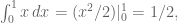
and we recover what we already know. In the next case, we need to integrate over two variables (same comment here, don’t have to divide by area of the 1×1 square base):

$\int_0^1 \int_0^1 max(x_1, x_2) \, dx_1 dx_2.$

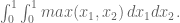
If you think about it, though, $x_1$ and $x_2$ play symmetric parts in this matter, so you can assume without loss of generality that $x_1$ is bigger, as long as we only let $x_2$ range between 0 and $x_1,$ and then multiply the end result by 2:

$= 2 \int_0^1 \int_0^{x_1} x_1 \, dx_2 dx_1.$

But that simplifies to:

$= 2 \int_0^1 x_1^2 \, dx = 2 (x_1^3/3) |_0^1 = 2/3.$

Let’s do the general case. It’s an n-fold integral over the maximum of all $n$ darts, and again without loss of generality $x_1$ is the maximum as long as we remember to multiply the whole thing by $n$ . We end up computing:

$= n \int_0^1 \int_0^{x_1} \int_0^{x_1} \cdots \int_0^{x_1} x_1 \, dx_n \cdots dx_3 dx_2 dx_1.$

But this collapses to:

$n \int_0^1 x_1^n \, dx_1 = n (x_1^{n+1}/(n+1)) |_0^1 = n/(n+1).$

To finish the original question, take the maximum value in your collection of draws and multiply it by the plumping factor $(n+1)/n$ to get a best estimate of the parameter $d.$

Categories: math, statistics

Comments (25)

Michael Edesess

October 13, 2013 at 8:26 am

I was just about to leave but saw this and couldn’t resist — sorry, haven’t actually read your post past the statement of the problem, but isn’t the maximum likelihood estimator of d just max x(i) itself? The probability that max x(i) is less than or equal to, say, y given d is (y/d)^n where n is the number of draws.

LikeLike
Mike Lawler

October 13, 2013 at 8:27 am

Wonderful explanation. I’m blown away by your ability to write these essays so quickly and clearly.

Perhaps as interesting as your problem, though, is how you apply it in practice – when is the assumption that you are seeing a draw from a uniform distribution (or whatever appropriate distribution) justified?

Suppose, for example, that you wanted to understand how often a company rated BBB+ by S&P files for bankruptcy. Looking at some historical data is probably a reasonable way to start.

However, when your favorite Wall St. sales team shows up at your door looking for a guarantee on a specific BBB+ rated company that they’ve selected, assuming this company was selected at random is going to get you in a load of trouble!

As an aside, the problem related to you problem, which Wikipedia calls the “Secretary Problem” is one of my favorites:

http://en.wikipedia.org/wiki/Secretary_problem

I first saw it in a neat book by Stephen Krantz called “Techniques of Problem Solving” where he works through it with numbers in envelopes.

LikeLike
Marcos

October 13, 2013 at 8:28 am

The book “Digital Dice: Computational Solutions to Practical Probability Problems” has a nice formulation of this problem, and its known as the German Tank problem ( http://en.wikipedia.org/wiki/German_tank_problem ).

LikeLike
JSE

October 13, 2013 at 10:07 am

What does “best guess for d” mean in this context? I mean, I get that you’re saying “expected value of max(x), given d, is dn/(n+1)” but it’s not totally obvious this translates into something I might mean by “best guess”, e.g. is it a maximum likelihood? Would this guess be licensed by a Bayesian reasoner under some reasonable prior on d? Is there a natural loss function where this estimate minimizes expected loss? I actually don’t even really get why it’s obvious that only max(x) matters. I’m sorry, I read something about the James Stein estimator (http://www-stat.stanford.edu/~omkar/329/chapter1.pdf) that blew my mind and it made me feel like I have to be super-pedantic about this stuff if I’m to have any hope of understanding it.

LikeLike
Tom

October 13, 2013 at 10:51 am

I’m with JSE. I think you have answered the much more interesting question about what is the likely max of a collection of numbers between 0 and d, but if you assume that the d itself was chosen, say, at random between 0 and N (or in fact according to any probability distribution which is nonincreasing) then I think it’s clear that the most likely value for d given a collection of samples x_i is just max(x_i), since a sample close to that one is more likely for smaller d, provided it is possible at all.

LikeLike
JSE

October 13, 2013 at 11:08 am

But I think this kind of reasoning is often raised as an objection to straight-up maximum likelihood arguments, because people like Cathy’s answer better than the d = max(x) answer!

LikeLike
- Cathy O'Neil, mathbabe
  
  October 13, 2013 at 11:26 am
  
  I agree with both of you of course, Jordan and Tom.
  
  If you think that d is actually arbitrary and that all we know about it is it’s positive, so say it’s taken from the uniform distribution from 0 to infinity, whatever that means, then after collecting lots of data points we know the most likely value for d is max(x_i), but it doesn’t mean that’s what we’d guess d is if we had to.
  
  One way to see this is by thinking discretely: if we had D sided-die and rolled it a bunch of times (n times, independently), then the likelihood of getting a given set of answers is always (1/D)^n. So as long as D is at least the maximum value, we can maximize the likelihood by minimizing D.
  
  Another way of saying this is that we can see that the distribution of d starts out pretty big, at max(x_i), and then dies really quickly, in fact exponentially quickly.
  
  I’d go with the plumped up version though if I were asked. I’ve so far avoided looking at references to think about this but I’d like to know how my “plumped up” version of max(x_i) relates to that distribution. It’s not the average value, for example, which is pretty easily computed to be log_{n+1}(2) max(x_i).
  
  LikeLike
  - Michael Hankin
    
    October 15, 2013 at 2:04 am
    
    Hi Cathy.
    Big fan of your blog. I think the approach you’ve taken is essentially the method of moments estimator (albeit the 1st moment of the max, a sufficient statistic, not the moment of the entire sample…). This underperforms the MLE in many cases, but in this case I think your approach is much more reasonable… though I can’t quite quantify why.
    
    LikeLike
    - Cathy O'Neil, mathbabe
      
      October 15, 2013 at 7:17 am
      
      Hey thanks, I was waiting for someone to come along who actually knows this stuff and could tell me what mess I’ve gotten myself into! 🙂
      
      LikeLike
Michael Edesess

October 13, 2013 at 11:03 pm

I have a feeling this must be the topic of a hundred math papers somewhere if you could find them. It’s an example of a problem where the maximum likelihood estimator result doesn’t feel right (it is max x(i), see for example http://ocw.mit.edu/courses/mathematics/18-443-statistics-for-applications-fall-2006/lecture-notes/lecture2.pdf). In fact it doesn’t even feel right to base the estimate only on max x(i). Shouldn’t the estimate be different if all the draws are bunched near max x(i) than if max x(i) is five times the second-highest draw?

LikeLike
- Cathy O'Neil, mathbabe
  
  October 14, 2013 at 6:34 am
  
  I agree it’s not yet satisfying. But as for your last question, no, since we are expected to believe it is actually uniform.
  
  LikeLike
Michael Edesess

October 14, 2013 at 6:45 am

Yes I see what you mean — it’s not intuitively obvious.

LikeLike
Guest2

October 14, 2013 at 8:43 am

This is where I lose you — “d” could be anything.

Is there a hidden assumption here that the distribution is smooth? monotonic? Because it may be non-linear, and then you’re screwed because your “best” guess may be worthless.

Same situation arises using the old P(n)+P(1)=>P(n+1) trick. It doesn’t work if [n, n+1] includes a bifurcation point.

LikeLike
JSE

October 14, 2013 at 9:09 am

OK I couldn’t sleep and thought about this a little more. The Bayesian way to do this would be to impose some prior distribution f on d; then the posterior, given your n observations with max(x(i)) = m, is going to be 0 for d = m. So what’s your “best guess” if that’s your distribution on d? Well, first of all, that depends on what f is. It can’t REALLY be “uniform distribution on the real numbers” but since that’s what you want f to be, let’s be fake Bayesians and say that’s what it is — after all, that gives us an honest distribution when n >= 2.

So with this distribution, what’s your “best guess” for d? Well, that depends on what your loss function is, I guess. If you’re trying to minimize expected squared error, then you want to pick the mean, which doesn’t exist for n <= 2 and otherwise is m(n-1)/(n-2), i.e the plump factor is (n-1)/(n-2). If you want to maximize chance of "being right," that's the same as maximum likelihood, which gives plump factor 1. (I think we all rightly reject this answer!) If you want to minimize expected absolute error I guess that amounts to taking the median of the distribution, which gives you a plump of 2^(1/(n-1)).

The plump of (n+1)/n is what you get if e.g. you take d to be distributed proportionally to d^{-2}.

I wonder which of these estimates, if any, people really think is "best"?

LikeLike
- Cathy O'Neil, mathbabe
  
  October 14, 2013 at 9:15 am
  
  Yes I’ve also been obsessed.
  
  I think it comes down to your “evaluation metric”. If you had a gameshow to make the best guess against other contestants, how would you decide the winner? It’s a nice thought experiment, and I might write a follow-up post, but in any case the “likelihood” estimate strategy wins the game on what is in fact a really terrible game show, whereas the various plumped-up versions win on game shows where the point is to get close to the right answer, for some definition of close.
  
  LikeLike
  - Mike Lawler
    
    October 14, 2013 at 11:19 am
    
    Funny enough there was a game show that is pretty close to what you describe.
    
    In 2003 and 2004 Pepsi ran a summer promotion called “Play for a Billion.” At the end of each summer, 1,000 winners of their contest were invited to be on a game show. Each contestant selected a six digit number from 000000 to 999999.
    
    After that, a special number was selected.
    
    Simplifying a little, if any of the contestants had selected the special number they would have one a $1 billion annuity (the present value was $250 million, I think). So you had 1,000 guesses from a set of 1,000,000 numbers.
    
    The contestant who was closest to the selected number would win $1 million. Here “close” was defined as having the most digits correct (with a few tie breakers).
    
    LikeLike
    - Cathy O'Neil, mathbabe
      
      October 14, 2013 at 12:48 pm
      
      Awesome! I totally hadn’t thought of that definition of close 🙂
      
      LikeLike
JSE

October 14, 2013 at 9:13 am

Hey look here’s a short exposition of exactly this!

http://www.amstat.org/publications/jse/v6n3/rossman.html

(n+1)/n is the “minimum variance unbiased estimator.”

LikeLike
Richard

October 14, 2013 at 2:06 pm

Cathy,

This is the ‘german tank’ problem. Google for it, you’ll find it.

Also interesting is to compare the accuracy of another approximation to your solition: d = 2*average(x). Etc, etc.

LikeLike
- Cathy O'Neil, mathbabe
  
  October 14, 2013 at 2:41 pm
  
  Richard,
  
  I know! But I’m trying to avoid looking at references until I have thoroughly thought about it myself! At some point I’ll break down and look, I’m sure.
  
  🙂
  
  Cathy
  
  LikeLike
  - Richard
    
    October 14, 2013 at 3:41 pm
    
    Cathy,
    
    Here is another problem.
    
    Same setting etc, etc, however now the numbers are generated by a (known) distribution.
    
    Or, even better, what if the numbers are generated by an unknown distribution?
    
    LikeLike
Stuart

October 15, 2013 at 8:09 am

I agree with lots of the comments above on the problems of defining what ‘best guess’ might be. This problem is a fun case where you can have lots of approaches that give interestingly different answers. You’re right that the number of observations and the largest observation are sufficient statistics (I think that’s the right terminology).

The largest observation is the max-likelihood estimate.

A Bayesian would need a prior, and probably a conjugate prior to make any analytical progress. The family of Pareto distributions is workable here.

You probably want to use an uninformative prior and the (improper) prior 1/d works well. The posterior is in the Pareto family and you can then read off percentiles from the posterior predictive.

You can seek a predictive interval rather than a confidence interval – e.g. seek an estimator d-hat such that you have a 95% (or 50% or whatever) probability of the next observation (not the unknown parameter! who cares about that?) falls below d-hat.

With the sufficient statistic to hand you can even follow Fisher’s fudicial probability approach and seek d-hat such that d has a 95% (etc) probability that d lies below d-hat. The fiducial distribution for d turns out to be Pareto too.

LikeLike
jmhl

October 16, 2013 at 11:19 pm

As mentioned by another commenter, this is known as the “German tank problem” and Wikipedia has an article giving a couple of approaches to it. E. T. Jaynes called this the “taxicab problem” and treats it very thoroughly from a Bayesian perspective in section 6.20 of his book “Probability Theory: The Logic Of Science.”

LikeLike
Stewart Gabory

October 18, 2013 at 9:05 pm

Some quick matlab/octave code to settle the issue once and for all:

NN = 100;
NTRIALS = 10000;
NESTIMATES = 4;
results = zeros(NTRIALS,NESTIMATES);

for ii = 1:NTRIALS
x = rand(1,NN);
results(ii,:) = [max(x), max(x)*(length(x)+1)/length(x), 2*mean(x), 2*median(x)];
end

bias = mean(results-1);
deviation = std(results);

Running it gives bias = [ -0.0100 -0.0001 0.0007 0.0009]
and deviation = [0.0097 0.0098 0.0575 0.0993]

So Cathy’s method appears to be unbiased with the least variance. Good enough for a lazy engineer.

LikeLike
- Cathy O'Neil, mathbabe
  
  October 19, 2013 at 8:14 am
  
  Nice, thanks! It’s all about the evaluation method.
  
  LikeLike