mathbabe

In the third week of the Columbia Data Science course, our guest lecturer was Jake Hofman. Jake is at Microsoft Research after recently leaving Yahoo! Research. He got a Ph.D. in physics at Columbia and taught a fantastic course on modeling last semester at Columbia.

After introducing himself, Jake drew up his “data science profile;” turns out he is an expert on a category that he created called “data wrangling.” He confesses that he doesn’t know if he spends so much time on it because he’s good at it or because he’s bad at it.

Thought Experiment: Learning by Example

Jake had us look at a bunch of text. What is it? After some time we describe each row as the subject and first line of an email in Jake’s inbox. We notice the bottom half of the rows of text looks like spam.

Now Jake asks us, how did you figure this out? Can you write code to automate the spam filter that your brain is?

Some ideas the students came up with:

• Any email is spam if it contains Viagra references. Jake: this will work if they don’t modify the word.
• Maybe something about the length of the subject?
• Exclamation points may point to spam. Jake: can’t just do that since “Yahoo!” would count.
• Jake: keep in mind spammers are smart. As soon as you make a move, they game your model. It would be great if we could get them to solve important problems.
• Should we use a probabilistic model? Jake: yes, that’s where we’re going.
• Should we use k-nearest neighbors? Should we use regression? Recall we learned about these techniques last week. Jake: neither. We’ll use Naive Bayes, which is somehow between the two.

Why is linear regression not going to work?

Say you make a feature for each lower case word that you see in any email and then we used R’s “lm function:”

lm(spam ~ word1 + word2 + …)

Wait, that’s too many variables compared to observations! We have on the order of 10,000 emails with on the order of 100,000 words. This will definitely overfit. Technically, this corresponds to the fact that the matrix in the equation for linear regression is not invertible. Moreover, maybe can’t even store it because it’s so huge.

Maybe you could limit to top 10,000 words? Even so, that’s too many variables vs. observations to feel good about it.

Another thing to consider is that target is 0 or 1 (0 if not spam, 1 if spam), whereas you wouldn’t get a 0 or a 1 in actuality through using linear regression, you’d get a number. Of course you could choose a critical value so that above that we call it “1” and below we call it “0”. Next week we’ll do even better when we explore logistic regression, which is set up to model a binary response like this.

How about k-nearest neighbors?

To use k-nearest neighbors we would still need to choose features, probably corresponding to words, and you’d likely define the value of those features to be 0 or 1 depending on whether the word is present or not. This leads to a weird notion of “nearness”.

Again, with 10,000 emails and 100,000 words, we’ll encounter a problem: it’s not a singular matrix this time but rather that the space we’d be working in has too many dimensions. This means that, for example, it requires lots of computational work to even compute distances, but even that’s not the real problem.

The real problem is even more basic: even your nearest neighbors are really far away. this is called “the curse of dimensionality“. This problem makes for a poor algorithm.

Question: what if sharing a bunch of words doesn’t mean sentences are near each other in the sense of language? I can imagine two sentences with the same words but very different meanings.

Jake: it’s not as bad as it sounds like it might be – I’ll give you references at the end that partly explain why.

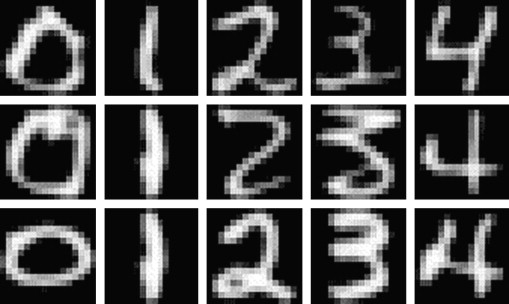
Aside: digit recognition

In this case k-nearest neighbors works well and moreover you can write it in a few lines of R.

Take your underlying representation apart pixel by pixel, say in a 16 x 16 grid of pixels, and measure how bright each pixel is. Unwrap the 16×16 grid and put it into a 256-dimensional space, which has a natural archimedean metric. Now apply the k-nearest neighbors algorithm.

Some notes:

• If you vary the number of neighbors, it changes the shape of the boundary and you can tune k to prevent overfitting.
• You can get 97% accuracy with a sufficiently large data set.
• Result can be viewed in a “confusion matrix“.

Naive Bayes

Question: You’re testing for a rare disease, with 1% of the population is infected. You have a highly sensitive and specific test:

• 99% of sick patients test positive
• 99% of healthy patients test negative

Given that a patient tests positive, what is the probability that the patient is actually sick?

Answer: Imagine you have 100×100 = 10,000 people. 100 are sick, 9,900 are healthy. 99 sick people test sick, and 99 healthy people do too. So if you test positive, you’re equally likely to be healthy or sick. So the answer is 50%.

Let’s do it again using fancy notation so we’ll feel smart:

Recall

and solve for

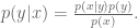
The denominator can be thought of as a “normalization constant;” we will often be able to avoid explicitly calculuating this. When we apply the above to our situation, we get:

This is called “Bayes’ Rule“. How do we use Bayes’ Rule to create a good spam filter? Think about it this way: if the word “Viagra” appears, this adds to the probability that the email is spam.

To see how this will work we will first focus on just one word at a time, which we generically call “word”. Then we have:

The right-hand side of the above is computable using enough pre-labeled data. If we refer to non-spam as “ham”, we only need and This is essentially a counting exercise.

Example: go online and download Enron emails. Awesome. We are building a spam filter on that – really this means we’re building a new spam filter on top of the spam filter that existed for the employees of Enron.

Jake has a quick and dirty shell script in bash which runs this. It downloads and unzips file, creates a folder. Each text file is an email. They put spam and ham in separate folders.

Jake uses “wc” to count the number of messages for one former Enron employee, for example. He sees 1500 spam, and 3672 ham. Using grep, he counts the number of instances of “meeting”:

grep -il meeting enron1/spam/*.txt | wc -l

This gives 153. This is one of the handful of computations we need to compute

Note we don’t need a fancy programming environment to get this done.

Next, we try:

• “money”: 80% chance of being spam.
• “viagra”: 100% chance.
• “enron”: 0% chance.

This illustrates overfitting; we are getting overconfident because of our biased data. It’s possible, in other words, to write an non-spam email with the word “viagra” as well as a spam email with the word “enron.”

Next, do it for all the words. Each document can be represented by a binary vector, whose jth entry is 1 or 0 depending whether jth word appears. Note this is a huge-ass vector, we will probably actually represent it with the indices of the words that actually do show up.

Here’s the model we use to estimate the probability that we’d see a given word vector given that we know it’s spam (or that it’s ham). We denote the document vector and the various entries , where the correspond to all the indices of in other words over all the words. For now we denote “is spam” by :

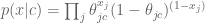
The theta here is the probability that an individual word is present in a spam email (we can assume separately and parallel-ly compute that for every word). Note we are modeling the words independently and we don’t count how many times they are present. That’s why this is called “Naive”.

Let’s take the log of both sides:

[It’s good to take the log because multiplying together tiny numbers can give us numerical problems.]

The term doesn’t depend on a given document, just the word, so let’s rename it Same with . The real weights that vary by document are the ‘s.

We can now use Bayes’ Rule to get an estimate of which is what we actually want. We can also get away with not computing all the terms if we only care whether it’s more likely to be spam or to be ham. Only the varying term needs to be computed.

Wait, this ends up looking like a linear regression! But instead of computing them by inverting a huge matrix, the weights come from the Naive Bayes’ algorithm.

This algorithm works pretty well and it’s “cheap to train” if you have pre-labeled data set to train on. Given a ton of emails, just count the words in spam and non-spam emails. If you get more training data you can easily increment your counts. In practice there’s a global model, which you personalize to individuals. Moreover, there are lots of hard-coded, cheap rules before an email gets put into a fancy and slow model.

Here are some references:

• “Idiot’s Bayes – not so stupid after all?” – the whole paper is about why it doesn’t suck, which is related to redundancies in language.
• “Naive Bayes at Forty: The Independence Assumption in Information“
• “Spam Filtering with Naive Bayes – Which Naive Bayes?“

Laplace Smoothing

Laplace Smoothing refers to the idea of replacing our straight-up estimate of the probability of seeing a given word in a spam email with something a bit fancier:

We might fix and for example, to prevents the possibility of getting 0 or 1 for a probability. Does this seem totally ad hoc? Well if we want to get fancy, we can see this as equivalent to having a prior and performing a maximal likelihood estimate.

If we denote by the maximal likelihood estimate, then we have:

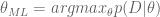
In other words, we are asking the question, for what value of were the data D most probable? If we assume independent trials then we want to maximize

If you take the derivative, and set it to zero, we get

In other words, just what we had before. Now let’s add a prior. Denote by the maximum a posteriori likelihood:

This similarly asks the question, given the data I saw, which parameter is the most likely?

Use Bayes’ rule to get . This looks similar to above except for the , which is the “prior”. If I assume is of the form ; then we get the above, Laplacian smoothed version.

Sometimes and are called “pseudo counts”. They’re fancy but also simple. It’s up to the data scientist to set the values of these hyperparameters, and it gives us two knobs to tune. By contrast, k-nearest neighbors has one knob, namely k.

Note: In the last 5 years people have started using stochastic gradient methods to avoid the non-invertible (overfitting) matrix problem. Switching to logistic regression with stochastic gradient method helped a lot, and can account for correlations between words. Even so, Naive Bayes’ is pretty impressively good considering how simple it is.

Scraping the web: API’s

For the sake of this discussion, an API (application programming interface) is something websites provide to developers so they can download data from the website easily and in standard format. Usually the developer has to register and receive a “key”, which is something like a password. For example, the New York Times has an API here. Note that some websites limit what data you have access to through their API’s or how often you can ask for data without paying for it.

When you go this route, you often get back weird formats, sometimes in JSON, but there’s no standardization to this standardization, i.e. different websites give you different “standard” formats.

One way to get beyond this is to use Yahoo’s YQL language which allows you to go to the Yahoo! Developer Network and write SQL-like queries that interact with many of the common API’s on the common sites like this:

select * from flickr.photos.search where text=”Cat” and api_key=”lksdjflskjdfsldkfj” limit 10

The output is standard and I only have to parse this in python once.

What if you want data when there’s no API available?

Note: always check the terms and services of the website before scraping.

In this case you might want to use something like the Firebug extension for Firefox, you can “inspect the element” on any webpage, and Firebug allows you to grab the field inside the html. In fact it gives you access to the full html document so you can interact and edit. In this way you can see the html as a map of the page and Firebug is a kind of tourguide.

After locating the stuff you want inside the html, you can use curl, wget, grep, awk, perl, etc., to write a quick and dirty shell script to grab what you want, especially for a one-off grab. If you want to be more systematic you can also do this using python or R.

Other parsing tools you might want to look into:

• lynx and lynx –dump: good if you pine for the 1970’s. Oh wait, 1992. Whatever.
• Beautiful Soup: robust but kind of slow
• Mechanize (or here) super cool as well but doesn’t parse javascript.

Postscript: Image Classification

How do you determine if an image is a landscape or a headshot?

You either need to get someone to label these things, which is a lot of work, or you can grab lots of pictures from flickr and ask for photos that have already been tagged.

Represent each image with a binned RGB – (red green blue) intensity histogram. In other words, for each pixel, for each of red, green, and blue, which are the basic colors in pixels, you measure the intensity, which is a number between 0 and 255.

Then draw three histograms, one for each basic color, showing us how many pixels had which intensity. It’s better to do a binned histogram, so have counts of # pixels of intensity 0 – 51, etc. – in the end, for each picture, you have 15 numbers, corresponding to 3 colors and 5 bins per color. We are assuming every picture has the same number of pixels here.

Finally, use k-nearest neighbors to decide how much “blue” makes a landscape versus a headshot. We can tune the hyperparameters, which in this case are # of bins as well as k.